1. Seurat Seurat Tabula Muris Analysis
Valeria Policastro
2025-12-10
Source:vignettes/RobinSingleCellVignetteNew.Rmd
RobinSingleCellVignetteNew.RmdSingle cell RNAseq Analysis
Reading data
# datav2 <- system.file("extdata", "filtered_tabulamuris_mtx.rds", package="scrobinv2")
datav2 <- get_data_path("filtered_tabulamuris_mtx.rds")
tabData <- readRDS(file=datav2)

SingleCellData <- CreateSeuratObject(counts = tabData, project = "singleCell", min.cells = round(dim(tabData)[2]*5/100), min.features = 0)
SingleCellData
## An object of class Seurat
## 8694 features across 532 samples within 1 assay
## Active assay: RNA (8694 features, 0 variable features)
## 1 layer present: countsData normalization
SingleCellData <- NormalizeData(SingleCellData, normalization.method = "LogNormalize", scale.factor = 10000)

SingleCellData[["RNA"]]@layers$counts[1:5,1:5]
## 5 x 5 sparse Matrix of class "dgCMatrix"
##
## [1,] . . . . .
## [2,] . . 1 . 1
## [3,] . . 1 . 1
## [4,] 1 . 1 . .
## [5,] 1 1 2 . .Feature selection
SingleCellData <- FindVariableFeatures(object = SingleCellData, selection.method="vst", nfeatures = 2000)Scale the data
SingleCellData <- ScaleData(SingleCellData, do.center = TRUE, do.scale = TRUE)
SingleCellData[["RNA"]]@layers$scale.data[1:5,1:5]
## [,1] [,2] [,3] [,4] [,5]
## [1,] -0.2119967 -0.2119967 -0.2119967 -0.2119967 -0.2119967
## [2,] -0.2464207 -0.2464207 -0.2464207 6.4241312 -0.2464207
## [3,] -0.2325839 -0.2325839 -0.2325839 -0.2325839 -0.2325839
## [4,] -0.3036820 -0.3036820 -0.3036820 -0.3036820 -0.3036820
## [5,] -0.2199427 -0.2199427 -0.2199427 -0.2199427 -0.2199427Linear dimension reduction
SingleCellData <- RunPCA(SingleCellData, features = VariableFeatures(object = SingleCellData))Graph
SingleCellData <- FindNeighbors(SingleCellData, dims = 1:50)

SingleCellData@graphs$RNA_snn[1:5,1:5] # Adjacency matrix
## 5 x 5 sparse Matrix of class "dgCMatrix"
## 10X_P4_7_CCTACACGTAAGGATT 10X_P7_6_ACACCGGGTAGCGTGA
## 10X_P4_7_CCTACACGTAAGGATT 1.0000000 0.1428571
## 10X_P7_6_ACACCGGGTAGCGTGA 0.1428571 1.0000000
## 10X_P7_9_TGATTTCAGCAGGTCA . .
## 10X_P8_14_CGAATGTAGAAGGTGA . .
## 10X_P4_6_CGATGGCCATCACAAC . .
## 10X_P7_9_TGATTTCAGCAGGTCA 10X_P8_14_CGAATGTAGAAGGTGA
## 10X_P4_7_CCTACACGTAAGGATT . .
## 10X_P7_6_ACACCGGGTAGCGTGA . .
## 10X_P7_9_TGATTTCAGCAGGTCA 1.0000000 .
## 10X_P8_14_CGAATGTAGAAGGTGA . 1
## 10X_P4_6_CGATGGCCATCACAAC 0.2121212 .
## 10X_P4_6_CGATGGCCATCACAAC
## 10X_P4_7_CCTACACGTAAGGATT .
## 10X_P7_6_ACACCGGGTAGCGTGA .
## 10X_P7_9_TGATTTCAGCAGGTCA 0.2121212
## 10X_P8_14_CGAATGTAGAAGGTGA .
## 10X_P4_6_CGATGGCCATCACAAC 1.0000000How to use Robin
Reading Graph
AdjSNN <- SingleCellData@graphs$RNA_snn
graphSingleCell <- graph_from_adjacency_matrix(AdjSNN,mode="directed",weighted = TRUE,add.colnames = "NA",diag=FALSE)
edge <- as_edgelist(graphSingleCell)
graph <- igraph::graph_from_edgelist(edge, directed=FALSE)
graph <- igraph::simplify(graph)
graph
## IGRAPH 7b0fe81 U--- 532 14421 --
## + edges from 7b0fe81:
## [1] 1-- 2 1-- 8 1-- 13 1-- 14 1-- 17 1-- 27 1-- 42 1-- 63 1-- 65 1-- 71
## [11] 1-- 79 1-- 95 1-- 99 1--102 1--116 1--131 1--132 1--159 1--161 1--164
## [21] 1--172 1--179 1--194 1--197 1--205 1--220 1--258 1--260 1--264 1--267
## [31] 1--270 1--312 1--315 1--325 1--327 1--328 1--351 1--368 1--378 1--386
## [41] 1--391 1--393 1--395 1--397 1--406 1--407 1--409 1--420 1--421 1--426
## [51] 1--427 1--432 1--452 1--458 1--459 1--464 1--472 1--473 1--476 1--478
## [61] 1--495 1--496 1--497 1--501 1--502 1--503 1--510 1--518 2-- 8 2-- 13
## [71] 2-- 14 2-- 27 2-- 42 2-- 63 2-- 65 2-- 71 2-- 79 2-- 95 2-- 99 2--102
## [81] 2--116 2--131 2--132 2--159 2--161 2--164 2--172 2--179 2--194 2--197
## + ... omitted several edgesCompare all algorithms vs Louvain
We apply the compare procedure to see which is the algorithm that better fits our network.
#Infomap
 comp_I <- robinCompare(graph=graph, method1="louvain",
                        method2="infomap")
## [1] "Unweighted Network Parallel Function"
## Detected robin method type independent
## It can take time ... It depends on the size of the network.
 plot1 <- plot(comp_I)


#Walktrap
comp_W <- robinCompare(graph=graph, method1="louvain",
                       method2="walktrap")
## [1] "Unweighted Network Parallel Function"
## Detected robin method type independent
## It can take time ... It depends on the size of the network.
plot2 <- plot(comp_W)


#LabelProp
comp_La <- robinCompare(graph=graph, method1="louvain",
                        method2="labelProp")
## [1] "Unweighted Network Parallel Function"
## Detected robin method type independent
## It can take time ... It depends on the size of the network.
plot3 <- plot(comp_La)

#Fastgreedy
comp_F <- robinCompare(graph=graph, method1="louvain",
                        method2="fastGreedy")
## [1] "Unweighted Network Parallel Function"
## Detected robin method type independent
## It can take time ... It depends on the size of the network.
plot4 <- plot(comp_F)


PlotComparisonAllVsInfomap <- gridExtra::grid.arrange(plot1,plot2,plot3,plot4, ncol=2)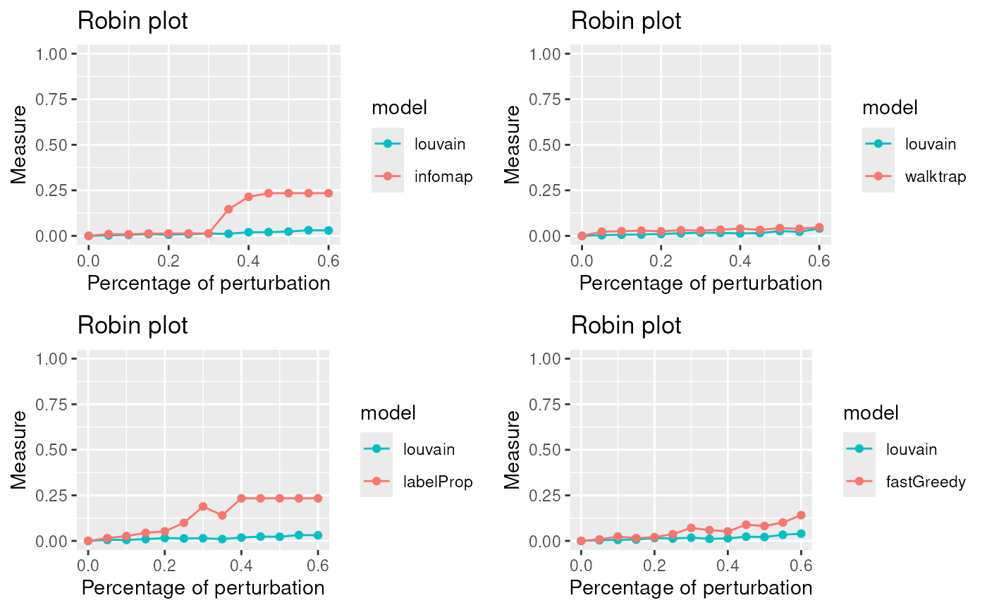
The lowest curve is the most stable algorithm. Louvain and Walktrap are the best algorithms in our example.
Statistical significance of communities
Due to the fact that Louvain is one of the best algorithm for our network we apply the robust procedure with the Louvain algorithm to see if the communities detected are statistically significant.
graphRandom <- random(graph=graph)
proc <- robinRobust(graph=graph, graphRandom=graphRandom, method="louvain")
## [1] "Unweighted Network Parallel Function"
## Detected robin method type independent
## It can take time ... It depends on the size of the network.
plot(proc)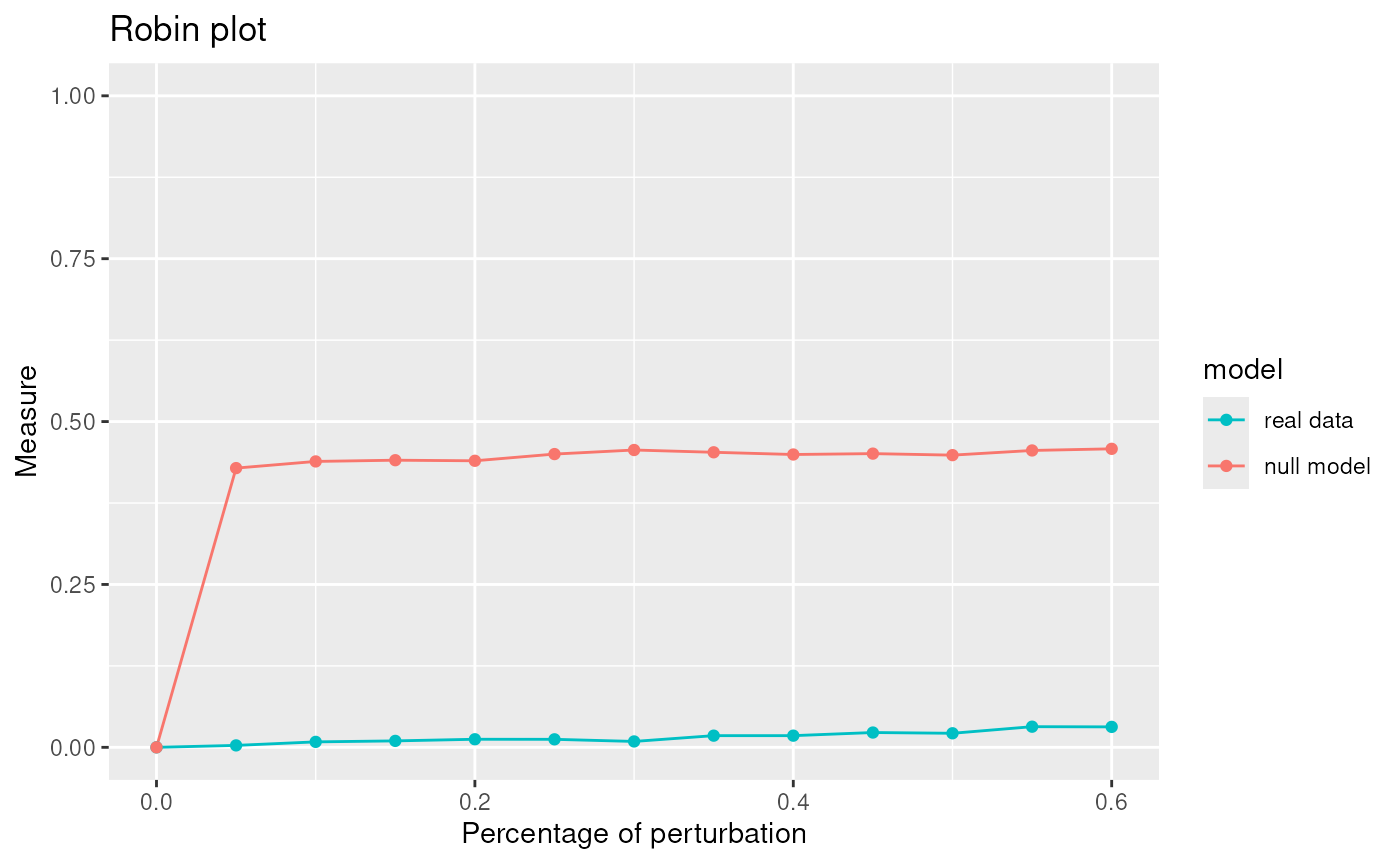
robinFDATest(proc)## [1] "First step: basis expansion"
## Swapping 'y' and 'argvals', because 'y' is simpler,
## and 'argvals' should be; now dim(argvals) = 13 ; dim(y) = 13 x 20
## [1] "Second step: joint univariate tests"
## [1] "Third step: interval-wise combination and correction"
## [1] "creating the p-value matrix: end of row 2 out of 9"
## [1] "creating the p-value matrix: end of row 3 out of 9"
## [1] "creating the p-value matrix: end of row 4 out of 9"
## [1] "creating the p-value matrix: end of row 5 out of 9"
## [1] "creating the p-value matrix: end of row 6 out of 9"
## [1] "creating the p-value matrix: end of row 7 out of 9"
## [1] "creating the p-value matrix: end of row 8 out of 9"
## [1] "creating the p-value matrix: end of row 9 out of 9"
## [1] "Interval Testing Procedure completed"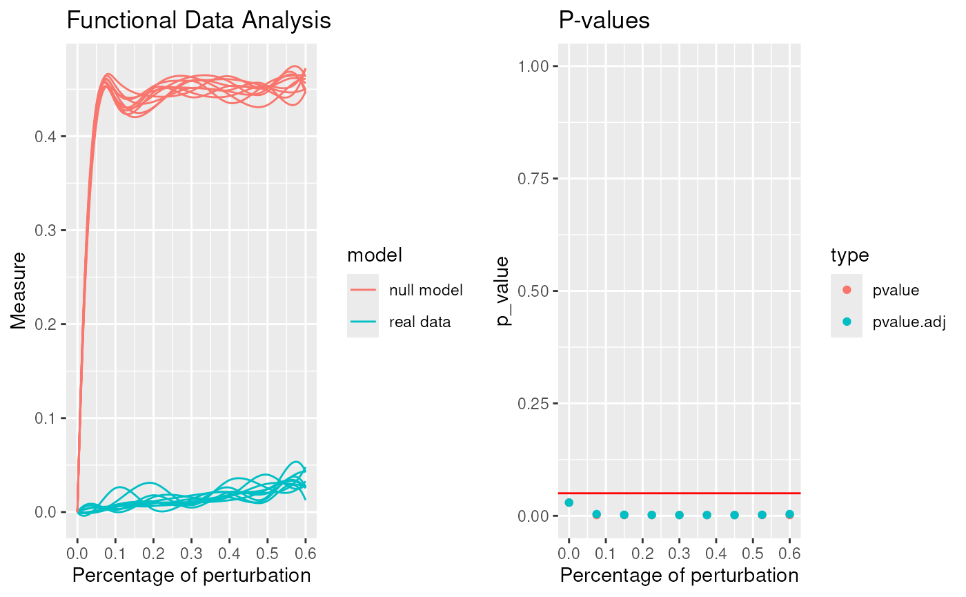
## TableGrob (1 x 2) "arrange": 2 grobs
##   z     cells    name           grob
## 1 1 (1-1,1-1) arrange gtable[layout]
## 2 2 (1-1,2-2) arrange gtable[layout]
## $adj.pvalue
## [1] 0.0102 0.0043 0.0022 0.0022 0.0022 0.0022 0.0022 0.0022 0.0024
##
## $pvalues
## [1] 0.0102 0.0022 0.0022 0.0022 0.0022 0.0022 0.0022 0.0022 0.0022
robinGPTest(proc)## Profile 1
## Profile 2## [1] 80.81106The communities given by Louvain are statistically significant.
Differential Analysis (Marker Gene Identification)
Once we found the best clustering algorithm, we can use the found communities for identifying marker genes, to subsequently find cell types.
mc <- membershipCommunities(graph=graph, method="louvain")
SingleCellData$seurat_clusters = mc
Idents(SingleCellData) <- "seurat_clusters"
markers <- FindAllMarkers(SingleCellData, only.pos = TRUE, logfc.threshold = 0.25)

markers %>%
    group_by(cluster) %>%
    dplyr::filter(avg_log2FC > 1) %>%
    slice_head(n = 10) %>%
    ungroup() -> top10
DoHeatmap(SingleCellData, features = top10$gene) + NoLegend()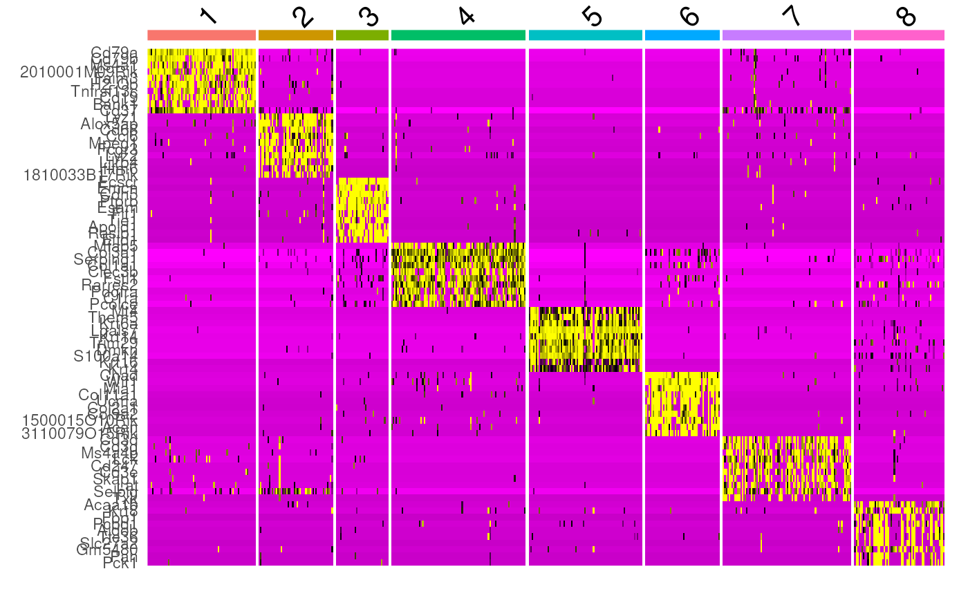
SessionInfo
## R version 4.4.2 (2024-10-31)
## Platform: x86_64-pc-linux-gnu
## Running under: Ubuntu 24.04.1 LTS
##
## Matrix products: default
## BLAS:   /usr/lib/x86_64-linux-gnu/openblas-pthread/libblas.so.3
## LAPACK: /usr/lib/x86_64-linux-gnu/openblas-pthread/libopenblasp-r0.3.26.so;  LAPACK version 3.12.0
##
## locale:
##  [1] LC_CTYPE=en_US.UTF-8       LC_NUMERIC=C
##  [3] LC_TIME=en_US.UTF-8        LC_COLLATE=en_US.UTF-8
##  [5] LC_MONETARY=en_US.UTF-8    LC_MESSAGES=en_US.UTF-8
##  [7] LC_PAPER=en_US.UTF-8       LC_NAME=C
##  [9] LC_ADDRESS=C               LC_TELEPHONE=C
## [11] LC_MEASUREMENT=en_US.UTF-8 LC_IDENTIFICATION=C
##
## time zone: Etc/UTC
## tzcode source: system (glibc)
##
## attached base packages:
## [1] stats     graphics  grDevices utils     datasets  methods   base
##
## other attached packages:
## [1] future_1.68.0      robin_2.0.0        igraph_2.2.1       mclust_6.1.2
## [5] patchwork_1.3.2    Seurat_5.3.1       SeuratObject_5.2.0 sp_2.2-0
## [9] dplyr_1.1.4
##
## loaded via a namespace (and not attached):
##   [1] RcppAnnoy_0.0.22       splines_4.4.2          later_1.4.4
##   [4] bitops_1.0-9           tibble_3.3.0           cellranger_1.1.0
##   [7] polyclip_1.10-7        fastDummies_1.7.5      deSolve_1.40
##  [10] lifecycle_1.0.4        globals_0.18.0         lattice_0.22-7
##  [13] MASS_7.3-65            magrittr_2.0.4         limma_3.62.2
##  [16] plotly_4.11.0          sass_0.4.10            rmarkdown_2.30
##  [19] jquerylib_0.1.4        yaml_2.3.11            httpuv_1.6.16
##  [22] otel_0.2.0             sctransform_0.4.2      spam_2.11-1
##  [25] askpass_1.2.1          spatstat.sparse_3.1-0  reticulate_1.44.1
##  [28] gld_2.6.8              cowplot_1.2.0          pbapply_1.7-4
##  [31] RColorBrewer_1.1-3     abind_1.4-8            expm_1.0-0
##  [34] Rtsne_0.17             purrr_1.2.0            RCurl_1.98-1.17
##  [37] pracma_2.4.6           data.tree_1.2.0        ggrepel_0.9.6
##  [40] irlba_2.3.5.1          listenv_0.10.0         spatstat.utils_3.2-0
##  [43] goftest_1.2-3          RSpectra_0.16-2        spatstat.random_3.4-3
##  [46] fitdistrplus_1.2-4     parallelly_1.45.1      pkgdown_2.2.0
##  [49] codetools_0.2-20       tidyselect_1.2.1       farver_2.1.2
##  [52] matrixStats_1.5.0      spatstat.explore_3.6-0 jsonlite_2.0.0
##  [55] e1071_1.7-16           ks_1.15.1              progressr_0.18.0
##  [58] ggridges_0.5.7         survival_3.8-3         systemfonts_1.3.1
##  [61] tools_4.4.2            ragg_1.5.0             DescTools_0.99.60
##  [64] ica_1.0-3              Rcpp_1.1.0             glue_1.8.0
##  [67] gridExtra_2.3          xfun_0.54              withr_3.0.2
##  [70] formatR_1.14           fastmap_1.2.0          boot_1.3-32
##  [73] digest_0.6.39          R6_2.6.1               mime_0.13
##  [76] qpdf_1.4.1             textshaping_1.0.4      colorspace_2.1-2
##  [79] networkD3_0.4.1        scattermore_1.2        tensor_1.5.1
##  [82] spatstat.data_3.1-9    tidyr_1.3.1            generics_0.1.4
##  [85] data.table_1.17.8      class_7.3-23           httr_1.4.7
##  [88] htmlwidgets_1.6.4      uwot_0.2.4             pkgconfig_2.0.3
##  [91] gtable_0.3.6           Exact_3.3              lmtest_0.9-40
##  [94] S7_0.2.1               pcaPP_2.0-5            htmltools_0.5.9
##  [97] dotCall64_1.2          scales_1.4.0           perturbR_0.1.3
## [100] lmom_3.2               png_0.1-8              spatstat.univar_3.1-5
## [103] knitr_1.50             rstudioapi_0.17.1      tzdb_0.5.0
## [106] reshape2_1.4.5         nlme_3.1-168           proxy_0.4-27
## [109] cachem_1.1.0           zoo_1.8-14             stringr_1.6.0
## [112] rootSolve_1.8.2.4      KernSmooth_2.23-26     parallel_4.4.2
## [115] miniUI_0.1.2           fda_6.3.0              desc_1.4.3
## [118] pillar_1.11.1          grid_4.4.2             vctrs_0.6.5
## [121] RANN_2.6.2             promises_1.5.0         xtable_1.8-4
## [124] cluster_2.1.8.1        evaluate_1.0.5         readr_2.1.6
## [127] mvtnorm_1.3-3          cli_3.6.5              compiler_4.4.2
## [130] rlang_1.1.6            fdatest_2.1.1          future.apply_1.20.0
## [133] labeling_0.4.3         fds_1.8                plyr_1.8.9
## [136] forcats_1.0.1          fs_1.6.6               stringi_1.8.7
## [139] rainbow_3.8            viridisLite_0.4.2      deldir_2.0-4
## [142] BiocParallel_1.40.2    hdrcde_3.4             lazyeval_0.2.2
## [145] spatstat.geom_3.6-1    Matrix_1.7-4           RcppHNSW_0.6.0
## [148] hms_1.1.4              ggplot2_4.0.1          statmod_1.5.1
## [151] shiny_1.12.0           haven_2.5.5            ROCR_1.0-11
## [154] bslib_0.9.0            readxl_1.4.5