2. OSCA Tabula Muris Analysis
Dario Righelli
2025-12-10
Source:vignettes/OSCATabulaMuris.Rmd
OSCATabulaMuris.RmdIntroduction
This document provides an analysis pipeline for Tabula Muris data using various R packages for single-cell RNA sequencing. Each chunk is annotated with a description of its purpose.
Load Required Libraries
The following libraries are loaded for data quality control, visualization, and analysis:
# Load necessary libraries for single-cell RNA-seq analysis
library(scater) # Data quality control and visualization
library(M3Drop) # Implements feature selection methods
library(Seurat) # Complete data analysis: QC, clustering, and exploration
library(mclust) # Metrics for clustering validation
library(scran) # Data preprocessing and normalization
library(SC3) # Clustering of scRNAseq data
library(SingleCellExperiment) # Core class for single-cell data
library(BiocParallel) # Parallel computation
library(HDF5Array) # Efficient storage and retrieval of HDF5 files
library(igraph)
library(robin)
Load Data
# Read data
# datav2 <- system.file("extdata", "filtered_tabulamuris_mtx.rds", package="scrobinv2")
datav2 <- get_data_path("filtered_tabulamuris_mtx.rds")
tabData <- readRDS(file=datav2)


# Read cell metadata
# inf <- system.file("extdata", "tabulamuris_cell_info.rds", package = "scrobinv2")
inf <- get_data_path("tabulamuris_cell_info.rds")
info1 <- readRDS(inf)
info <- subset(info1, id %in% colnames(tabData))
dim(info)
## [1] 532 7Create a SingleCellExperiment Object
Combine the data into a SingleCellExperiment object for downstream analysis:
# Create a SingleCellExperiment object
wrkrs <- 15 # Number of workers for parallelization
match_order <- match(colnames(tabData), rownames(info))
info <- info[match_order, ]
sce <- SingleCellExperiment(assays = list(counts = tabData), colData = info)
Quality Control
Add quality control metrics to the SingleCellExperiment object:
# Perform quality control and visualize cell metrics
sce <- addPerCellQC(sce)
hist(sce$total, breaks = 50, xlab = "Library Sizes", main = "Distribution of Library Sizes")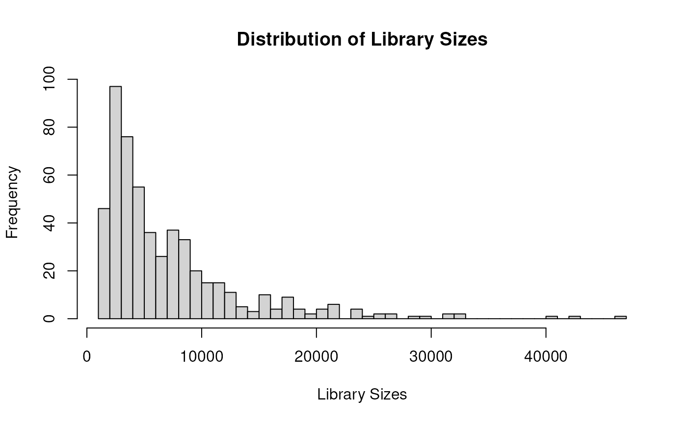
hist(sce$detected, xlab="Number of expressed genes", breaks=50, ylab="Number of cells")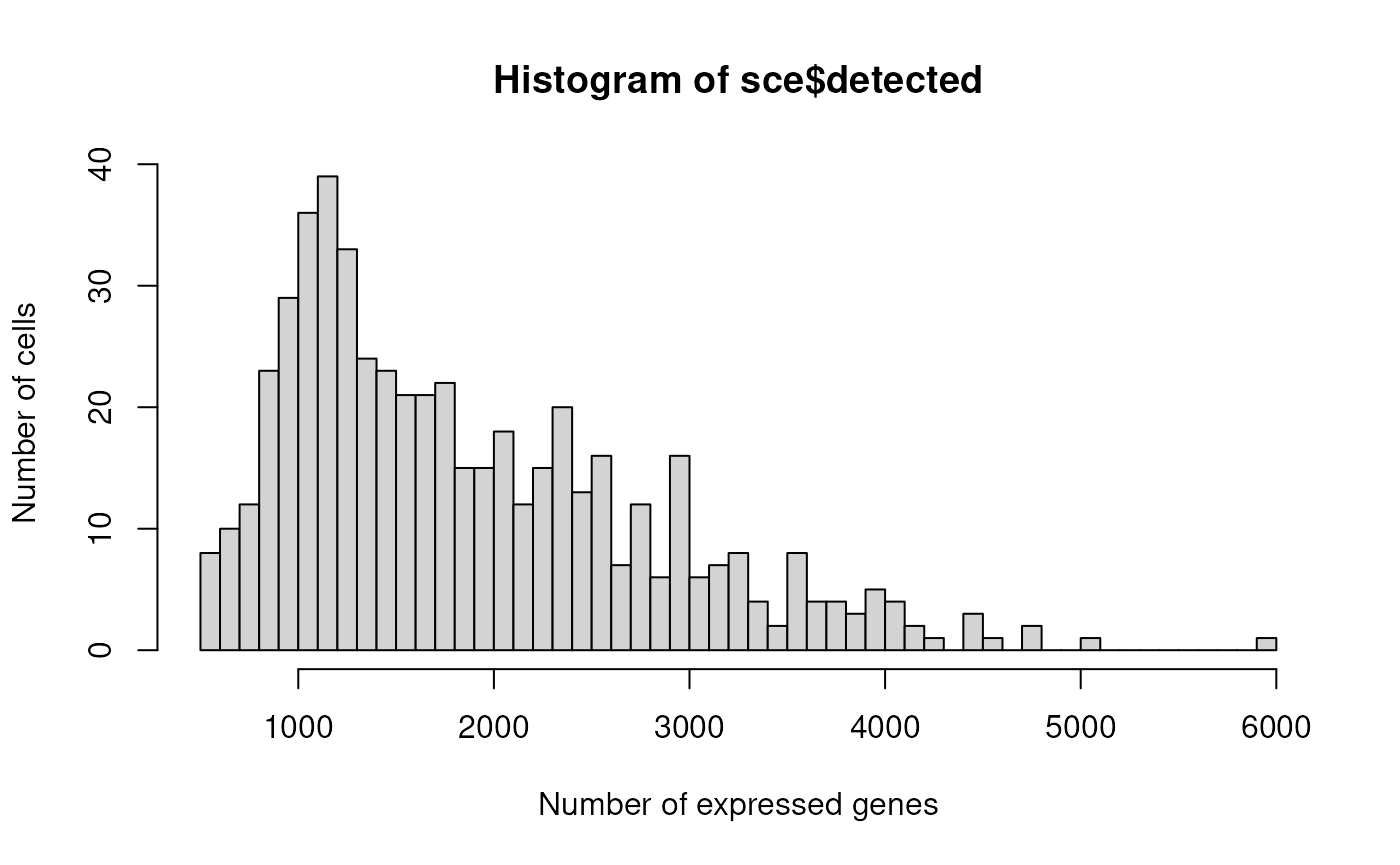
plotHighestExprs(sce, exprs_values = "counts")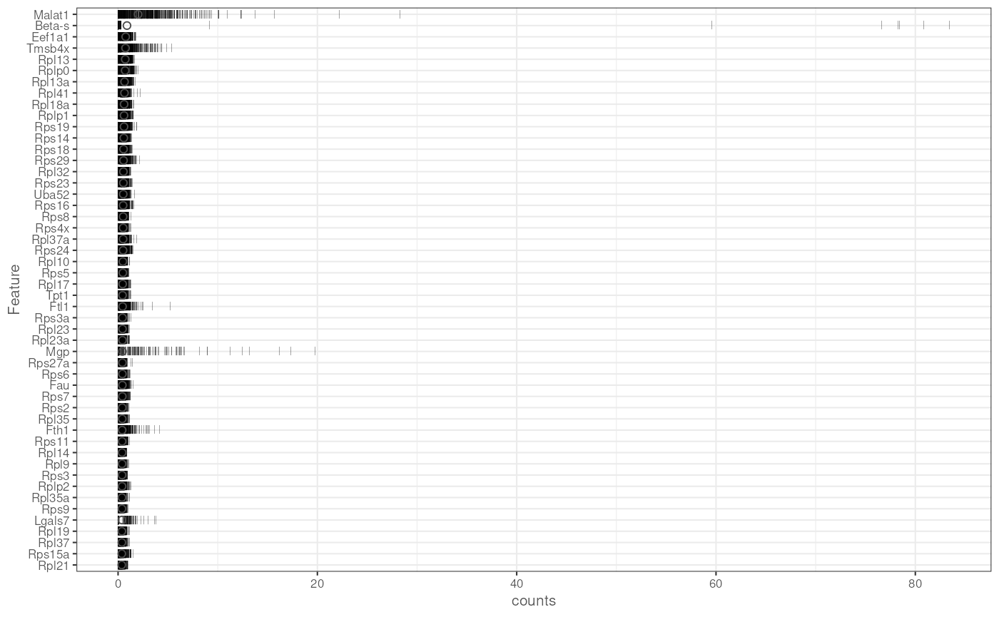
Filter Genes with Low Expression
Filter genes based on their average expression levels to exclude non-informative features.
# Calculate average counts for each gene and filter out genes with zero average expression
rowData(sce)$ave.counts <- calculateAverage(sce, exprs_values = "counts", BPPARAM = MulticoreParam(workers = wrkrs))
to.keep <- rowData(sce)$ave.counts > 0
sce <- sce[to.keep, ]
summary(to.keep)  # Summary of genes kept
## Mode FALSE TRUE
## logical 3571 16183
dim(sce) # Dimensions of the filtered SingleCellExperiment object## [1] 16183 532Normalize Counts
Normalize the data using scran’s computeSumFactors and log-normalization for downstream analysis.
# Compute size factors and normalize counts
set.seed(1000)
clusters <- quickCluster(sce, BPPARAM = MulticoreParam(workers = wrkrs))
sce <- computeSumFactors(sce, cluster = clusters, BPPARAM = MulticoreParam(workers = wrkrs))
sce <- logNormCounts(sce)
Variance Modelling and Highly Variable Genes
Model variance to identify highly variable genes for downstream analysis.
# Model variance and identify the top highly variable genes
set.seed(1001)
dec <- modelGeneVarByPoisson(sce, BPPARAM = MulticoreParam(workers = wrkrs))
top <- getTopHVGs(dec, prop = 0.1)
Dimensionality Reduction
Perform PCA, t-SNE, and UMAP for dimensionality reduction to visualize the data in lower-dimensional spaces.
# Perform PCA and reduce dimensions using t-SNE and UMAP
set.seed(10000)
sce <- denoisePCA(sce, subset.row = top, technical = dec, BPPARAM = MulticoreParam(workers = wrkrs))
ncol(reducedDim(sce))  # Number of principal components used
## [1] 18
set.seed(100000)
sce <- runTSNE(sce, dimred = "PCA")

set.seed(1000000)
sce <- runUMAP(sce, dimred = "PCA")
plotReducedDim(sce, dimred = "UMAP", colour_by = "cell_ontology_class")  # Plot UMAP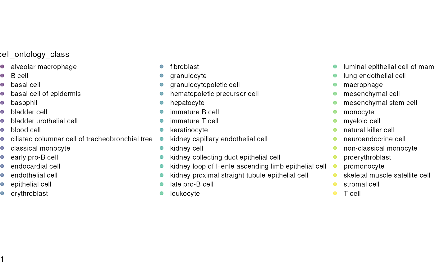
Graph Construction
Construct a shared nearest neighbor (SNN) graph based on PCA-reduced dimensions.
# Build a shared nearest neighbor (SNN) graph
graph <- buildSNNGraph(sce, k = 25, use.dimred = 'PCA')  # k=25 neighbors
Cluster Evaluation
Evaluate different clustering methods using robin
# Simplify the graph and evaluate clustering methods
graph <- igraph::simplify(graph) # Simplify the graph by removing duplicate edgesCompare all algorithms vs Louvain
We apply the compare procedure to see which is the algorithm that better fits our network.
library(robin)
graph <- prepGraph(graph, file.format="igraph")
#Infomap
 comp_I <- robinCompare(graph=graph, method1="louvain",
                        method2="infomap")
## [1] "Weighted Network Parallel Function"
## Detected robin method type independent
## It can take time ... It depends on the size of the network.
 plot1 <- plot(comp_I)


#Walktrap
comp_W <- robinCompare(graph=graph, method1="louvain",
                       method2="walktrap")
## [1] "Weighted Network Parallel Function"
## Detected robin method type independent
## It can take time ... It depends on the size of the network.
plot2 <- plot(comp_W)


#LabelProp
comp_La <- robinCompare(graph=graph, method1="louvain",
                        method2="labelProp") # use leiden
## [1] "Weighted Network Parallel Function"
## Detected robin method type independent
## It can take time ... It depends on the size of the network.
plot3 <- plot(comp_La)

#Fastgreedy
comp_F <- robinCompare(graph=graph, method1="louvain",
                        method2="fastGreedy")
## [1] "Weighted Network Parallel Function"
## Detected robin method type independent
## It can take time ... It depends on the size of the network.
plot4 <- plot(comp_F)


PlotComparisonAllVsInfomap <- gridExtra::grid.arrange(plot1,plot2,plot3,plot4, ncol=2)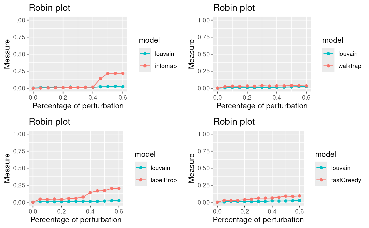
The lowest curve is the most stable algorithm. Louvain and Walktrap are the best algorithms in our example.
Statistical significance of communities
Due to the fact that Louvain is one of the best algorithm for our network we apply the robust procedure with the Louvain algorithm to see if the communities detected are statistically significant.
graphRandom <- random(graph=graph)
proc <- robinRobust(graph=graph, graphRandom=graphRandom, method="louvain")
## [1] "Weighted Network Parallel Function"
## Detected robin method type independent
## It can take time ... It depends on the size of the network.
plot(proc)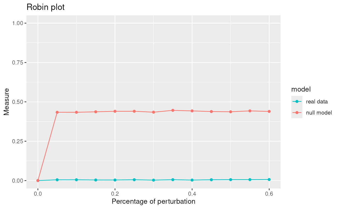
robinFDATest(proc)## [1] "First step: basis expansion"
## Swapping 'y' and 'argvals', because 'y' is simpler,
## and 'argvals' should be; now dim(argvals) = 13 ; dim(y) = 13 x 20
## [1] "Second step: joint univariate tests"
## [1] "Third step: interval-wise combination and correction"
## [1] "creating the p-value matrix: end of row 2 out of 9"
## [1] "creating the p-value matrix: end of row 3 out of 9"
## [1] "creating the p-value matrix: end of row 4 out of 9"
## [1] "creating the p-value matrix: end of row 5 out of 9"
## [1] "creating the p-value matrix: end of row 6 out of 9"
## [1] "creating the p-value matrix: end of row 7 out of 9"
## [1] "creating the p-value matrix: end of row 8 out of 9"
## [1] "creating the p-value matrix: end of row 9 out of 9"
## [1] "Interval Testing Procedure completed"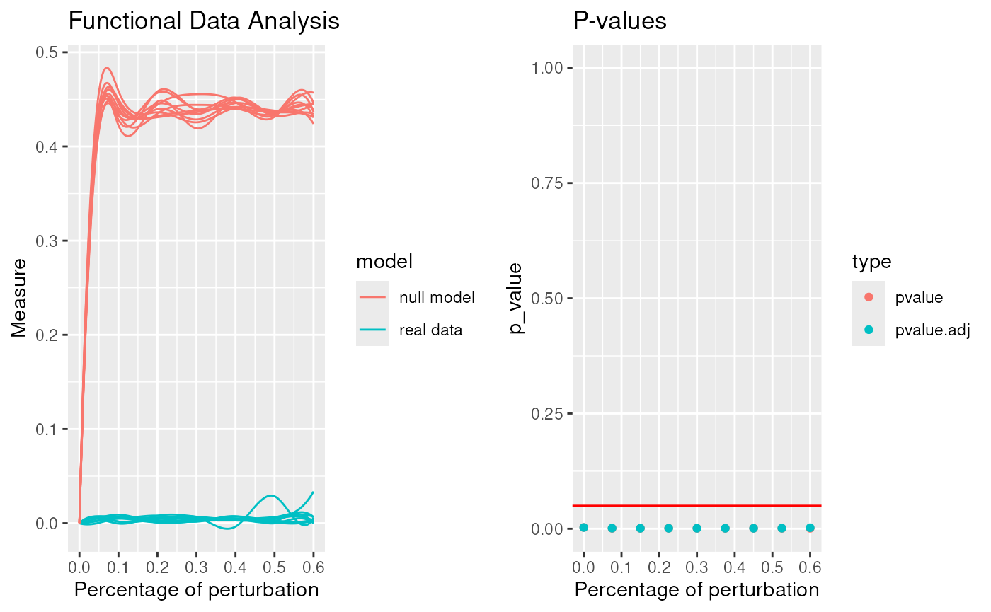
## TableGrob (1 x 2) "arrange": 2 grobs
##   z     cells    name           grob
## 1 1 (1-1,1-1) arrange gtable[layout]
## 2 2 (1-1,2-2) arrange gtable[layout]
## $adj.pvalue
## [1] 0.2822 0.0026 0.0010 0.0010 0.0010 0.0010 0.0010 0.0010 0.0013
##
## $pvalues
## [1] 0.2822 0.0010 0.0010 0.0010 0.0010 0.0010 0.0010 0.0010 0.0010
robinGPTest(proc)## Profile 1
## Profile 2## [1] 50.58246The communities given by Louvain are statistically significant.
Communities
table(membershipCommunities (graph=graph, method="louvain"))##
## 1 2 3 4 5 6
## 73 133 111 91 75 49Differential Analysis (Marker Gene Identification)
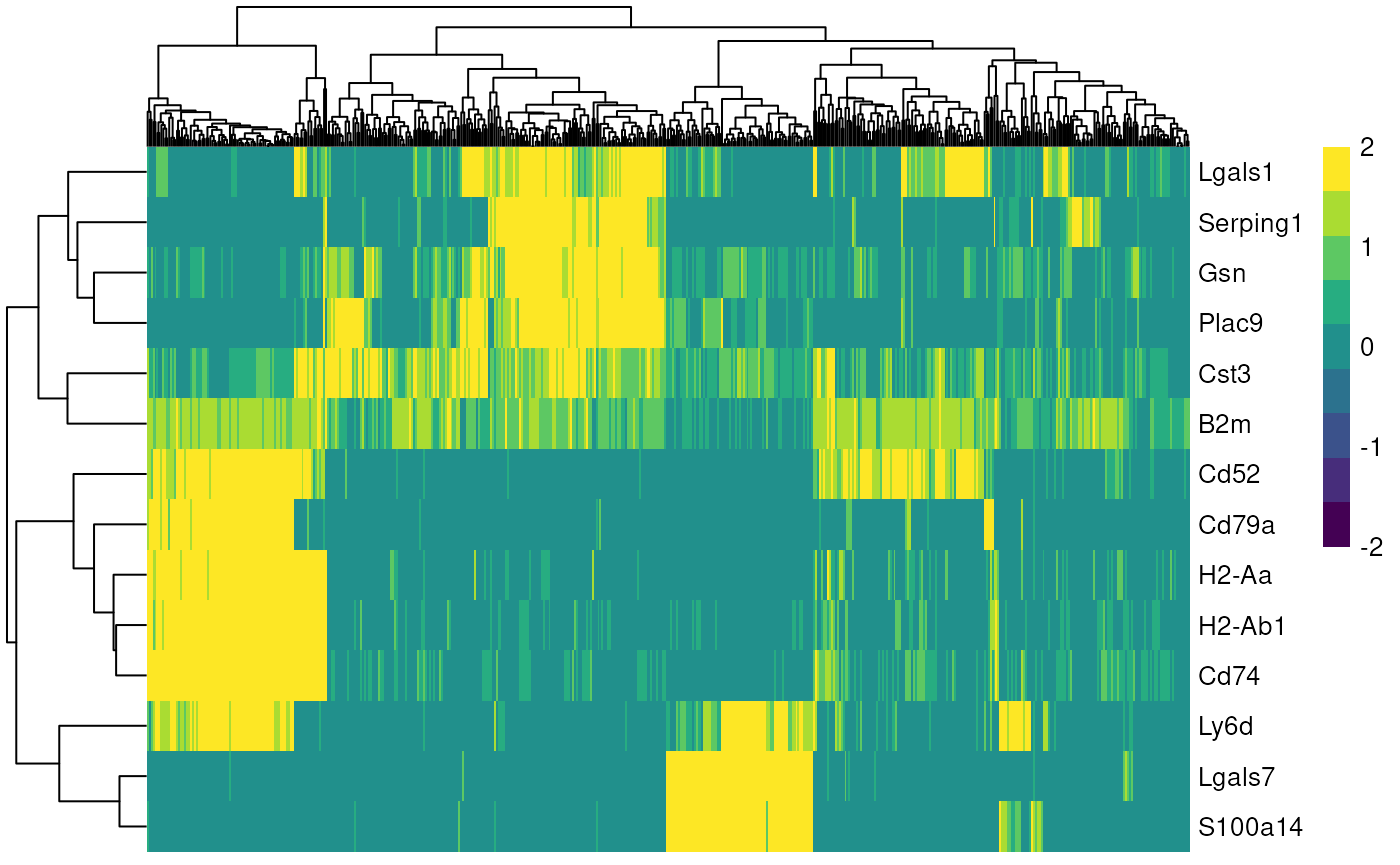
Once we found the best clustering algorithm, we can use the found communities for identifying marker genes, to subsequently find cell types.
mc <- membershipCommunities(graph=graph, method="louvain")

sce$louvain <- mc
markers <- findMarkers(sce, groups=sce$louvain)
marker_genes <- unique(unlist(lapply(markers, function(m) head(rownames(m), 5))))
plotHeatmap(
  sce,
  features = marker_genes,
  columns_by = "louvain",
  exprs_values = "logcounts",
  scale = TRUE,
  centre = TRUE,
  zlim = c(-2, 2)
)
Session Info
## R version 4.4.2 (2024-10-31)
## Platform: x86_64-pc-linux-gnu
## Running under: Ubuntu 24.04.1 LTS
##
## Matrix products: default
## BLAS:   /usr/lib/x86_64-linux-gnu/openblas-pthread/libblas.so.3
## LAPACK: /usr/lib/x86_64-linux-gnu/openblas-pthread/libopenblasp-r0.3.26.so;  LAPACK version 3.12.0
##
## locale:
##  [1] LC_CTYPE=en_US.UTF-8       LC_NUMERIC=C
##  [3] LC_TIME=en_US.UTF-8        LC_COLLATE=en_US.UTF-8
##  [5] LC_MONETARY=en_US.UTF-8    LC_MESSAGES=en_US.UTF-8
##  [7] LC_PAPER=en_US.UTF-8       LC_NAME=C
##  [9] LC_ADDRESS=C               LC_TELEPHONE=C
## [11] LC_MEASUREMENT=en_US.UTF-8 LC_IDENTIFICATION=C
##
## time zone: Etc/UTC
## tzcode source: system (glibc)
##
## attached base packages:
## [1] stats4    stats     graphics  grDevices utils     datasets  methods
## [8] base
##
## other attached packages:
##  [1] robin_2.0.0                 igraph_2.2.1
##  [3] HDF5Array_1.34.0            rhdf5_2.50.2
##  [5] DelayedArray_0.32.0         SparseArray_1.6.2
##  [7] S4Arrays_1.6.0              abind_1.4-8
##  [9] Matrix_1.7-4                BiocParallel_1.40.2
## [11] SC3_1.34.0                  scran_1.34.0
## [13] mclust_6.1.2                Seurat_5.3.1
## [15] SeuratObject_5.2.0          sp_2.2-0
## [17] M3Drop_1.32.0               numDeriv_2016.8-1.1
## [19] scater_1.34.1               ggplot2_4.0.1
## [21] scuttle_1.16.0              SingleCellExperiment_1.28.1
## [23] SummarizedExperiment_1.36.0 Biobase_2.66.0
## [25] GenomicRanges_1.58.0        GenomeInfoDb_1.42.3
## [27] IRanges_2.40.1              S4Vectors_0.44.0
## [29] BiocGenerics_0.52.0         MatrixGenerics_1.18.1
## [31] matrixStats_1.5.0
##
## loaded via a namespace (and not attached):
##   [1] gld_2.6.8                nnet_7.3-20              goftest_1.2-3
##   [4] rstan_2.32.7             vctrs_0.6.5              spatstat.random_3.4-3
##   [7] perturbR_0.1.3           digest_0.6.39            png_0.1-8
##  [10] proxy_0.4-27             Exact_3.3                pcaPP_2.0-5
##  [13] ggrepel_0.9.6            deldir_2.0-4             parallelly_1.45.1
##  [16] hdrcde_3.4               MASS_7.3-65              pkgdown_2.2.0
##  [19] reshape2_1.4.5           httpuv_1.6.16            foreach_1.5.2
##  [22] withr_3.0.2              xfun_0.54                survival_3.8-3
##  [25] doRNG_1.8.6.2            ggbeeswarm_0.7.3         systemfonts_1.3.1
##  [28] ragg_1.5.0               networkD3_0.4.1          zoo_1.8-14
##  [31] gtools_3.9.5             V8_8.0.1                 pbapply_1.7-4
##  [34] DEoptimR_1.1-4           Formula_1.2-5            promises_1.5.0
##  [37] otel_0.2.0               httr_1.4.7               globals_0.18.0
##  [40] fitdistrplus_1.2-4       rhdf5filters_1.18.1      rstudioapi_0.17.1
##  [43] UCSC.utils_1.2.0         miniUI_0.1.2             generics_0.1.4
##  [46] base64enc_0.1-3          curl_7.0.0               zlibbioc_1.52.0
##  [49] ScaledMatrix_1.14.0      polyclip_1.10-7          GenomeInfoDbData_1.2.13
##  [52] xtable_1.8-4             stringr_1.6.0            desc_1.4.3
##  [55] pracma_2.4.6             doParallel_1.0.17        evaluate_1.0.5
##  [58] hms_1.1.4                irlba_2.3.5.1            colorspace_2.1-2
##  [61] ROCR_1.0-11              reticulate_1.44.1        readxl_1.4.5
##  [64] spatstat.data_3.1-9      magrittr_2.0.4           lmtest_0.9-40
##  [67] readr_2.1.6              later_1.4.4              viridis_0.6.5
##  [70] lattice_0.22-7           spatstat.geom_3.6-1      future.apply_1.20.0
##  [73] robustbase_0.99-6        scattermore_1.2          cowplot_1.2.0
##  [76] RcppAnnoy_0.0.22         class_7.3-23             Hmisc_5.2-4
##  [79] pillar_1.11.1            StanHeaders_2.32.10      nlme_3.1-168
##  [82] iterators_1.0.14         caTools_1.18.3           compiler_4.4.2
##  [85] beachmat_2.22.0          RSpectra_0.16-2          stringi_1.8.7
##  [88] DescTools_0.99.60        tensor_1.5.1             plyr_1.8.9
##  [91] fda_6.3.0                crayon_1.5.3             locfit_1.5-9.12
##  [94] haven_2.5.5              rootSolve_1.8.2.4        dplyr_1.1.4
##  [97] codetools_0.2-20         textshaping_1.0.4        BiocSingular_1.22.0
## [100] bslib_0.9.0              QuickJSR_1.8.1           e1071_1.7-16
## [103] lmom_3.2                 fds_1.8                  plotly_4.11.0
## [106] mime_0.13                splines_4.4.2            Rcpp_1.1.0
## [109] fastDummies_1.7.5        sparseMatrixStats_1.18.0 cellranger_1.1.0
## [112] knitr_1.50               reldist_1.7-2            WriteXLS_6.8.0
## [115] fs_1.6.6                 listenv_0.10.0           checkmate_2.3.3
## [118] pkgbuild_1.4.8           expm_1.0-0               tibble_3.3.0
## [121] statmod_1.5.1            tzdb_0.5.0               pkgconfig_2.0.3
## [124] pheatmap_1.0.13          tools_4.4.2              cachem_1.1.0
## [127] viridisLite_0.4.2        fastmap_1.2.0            rmarkdown_2.30
## [130] scales_1.4.0             grid_4.4.2               ica_1.0-3
## [133] sass_0.4.10              FNN_1.1.4.1              patchwork_1.3.2
## [136] dotCall64_1.2            RANN_2.6.2               rpart_4.1.24
## [139] farver_2.1.2             mgcv_1.9-4               yaml_2.3.11
## [142] deSolve_1.40             foreign_0.8-90           cli_3.6.5
## [145] purrr_1.2.0              lifecycle_1.0.4          askpass_1.2.1
## [148] uwot_0.2.4               rainbow_3.8              mvtnorm_1.3-3
## [151] bluster_1.16.0           backports_1.5.0          gtable_0.3.6
## [154] ggridges_0.5.7           densEstBayes_1.0-2.2     progressr_0.18.0
## [157] parallel_4.4.2           limma_3.62.2             jsonlite_2.0.0
## [160] edgeR_4.4.2              RcppHNSW_0.6.0           bitops_1.0-9
## [163] Rtsne_0.17               spatstat.utils_3.2-0     BiocNeighbors_2.0.1
## [166] RcppParallel_5.1.11-1    bdsmatrix_1.3-7          jquerylib_0.1.4
## [169] metapod_1.14.0           dqrng_0.4.1              loo_2.8.0
## [172] spatstat.univar_3.1-5    rrcov_1.7-7              lazyeval_0.2.2
## [175] shiny_1.12.0             htmltools_0.5.9          sctransform_0.4.2
## [178] formatR_1.14             data.tree_1.2.0          glue_1.8.0
## [181] spam_2.11-1              XVector_0.46.0           RCurl_1.98-1.17
## [184] qpdf_1.4.1               ks_1.15.1                gridExtra_2.3
## [187] boot_1.3-32              R6_2.6.1                 tidyr_1.3.1
## [190] fdatest_2.1.1            gplots_3.3.0             labeling_0.4.3
## [193] forcats_1.0.1            cluster_2.1.8.1          rngtools_1.5.2
## [196] bbmle_1.0.25.1           Rhdf5lib_1.28.0          rstantools_2.5.0
## [199] tidyselect_1.2.1         vipor_0.4.7              htmlTable_2.4.3
## [202] inline_0.3.21            future_1.68.0            rsvd_1.0.5
## [205] KernSmooth_2.23-26       S7_0.2.1                 data.table_1.17.8
## [208] htmlwidgets_1.6.4        RColorBrewer_1.1-3       rlang_1.1.6
## [211] spatstat.sparse_3.1-0    spatstat.explore_3.6-0   beeswarm_0.4.0