3. OSCA Human Improved Analysis
Dario Righelli
2025-12-10
Source:vignettes/OSCA_SCMM.Rmd
OSCA_SCMM.RmdIntroduction
This document provides an analysis pipeline for single cell RNAseq of a multimodal dataset from the SingleCellMultimodl Bioconductor package using various R packages for single-cell RNA sequencing. Each chunk is annotated with a description of its purpose.
Load Required Libraries
The following libraries are loaded for data quality control, visualization, and analysis:
# Load necessary libraries for single-cell RNA-seq analysis
library(scater) # Data quality control and visualization
library(BiocParallel) # Parallel computation
library(scran) # Data preprocessing and normalization
library(igraph) # graph handling
library(ggplot2) # visualization
library(SingleCellExperiment) # Core class for single-cell data
library(SingleR) # annotation of cell types
library(celldex) # reference dataset
library(bluster) #
library(robin)
library(reshape2)
Load Data
For lack of time, we saved the sce in a dedicated object.
library(SingleCellMultiModal)

mae <- SingleCellMultiModal::scMultiome(dry.run=FALSE)
sce <- mae@ExperimentList$rna
sce
Additionally, we load an object with already computed PCA/TSNE/UMAP dimentionality reductions.
scev2 <- get_data_path("scescmm.rds")
sce <- readRDS(scev2)
Quality Control
Add quality control metrics to the SingleCellExperiment object:
# Perform quality control and visualize cell metrics
sce <- addPerCellQC(sce)
hist(sce$total, breaks = 50, xlab = "Library Sizes", main = "Distribution of Library Sizes")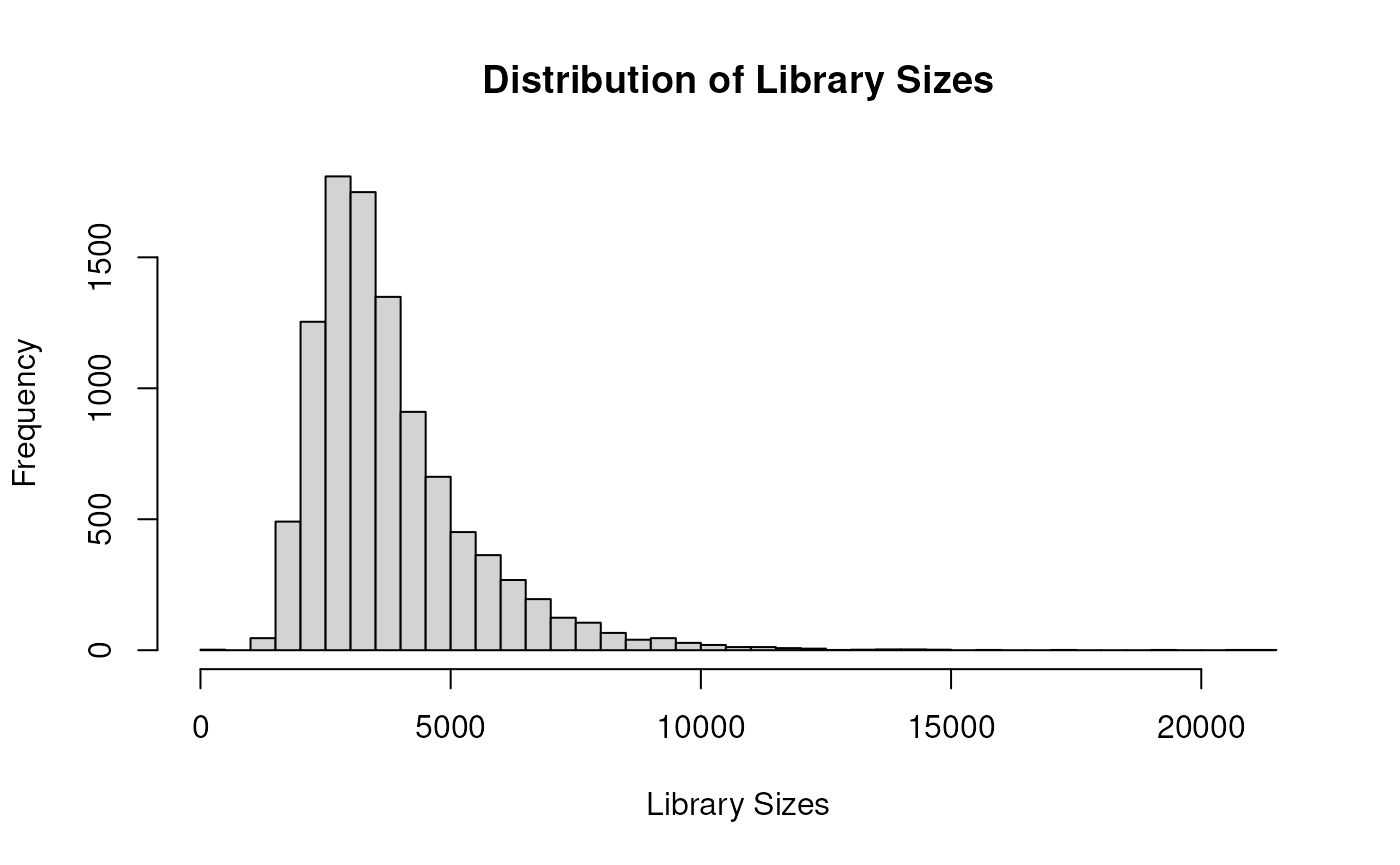
hist(sce$detected, xlab="Number of expressed genes", breaks=50, ylab="Number of cells")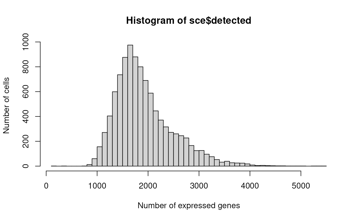
plotHighestExprs(sce, exprs_values = "counts")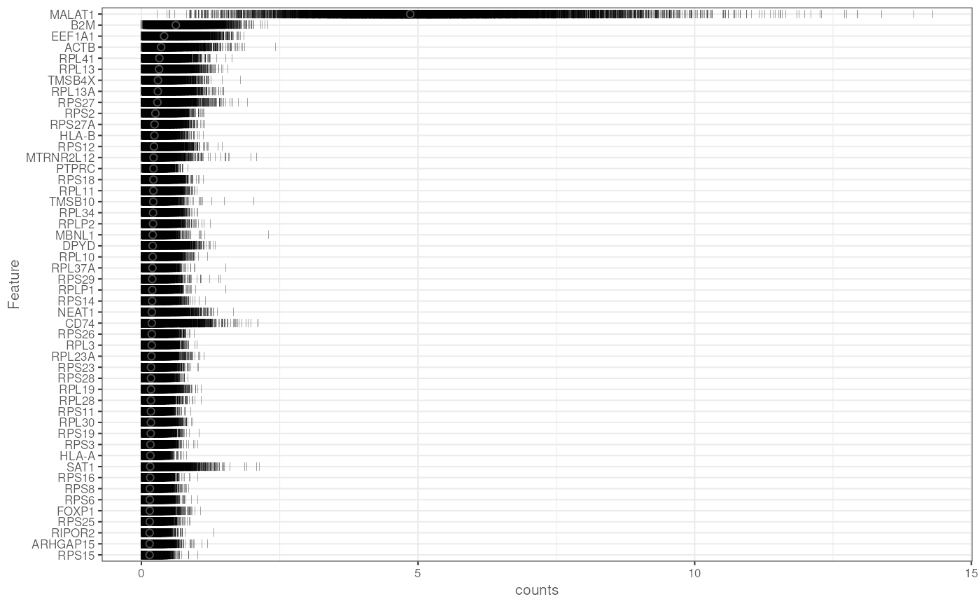
Filter Genes with Low Expression
Filter genes based on their average expression levels to exclude non-informative features.
wrkrs <- 15
# Calculate average counts for each gene and filter out genes with zero average expression
rowData(sce)$ave.counts <- calculateAverage(sce, exprs_values = "counts", BPPARAM = MulticoreParam(workers = wrkrs))
to.keep <- rowData(sce)$ave.counts > 0
sce <- sce[to.keep, ]
summary(to.keep)  # Summary of genes kept
## Mode TRUE
## logical 29100
dim(sce) # Dimensions of the filtered SingleCellExperiment object## [1] 29100 10032Normalize Counts
Normalize the data using scran’s computeSumFactors and log-normalization for downstream analysis.
set.seed(1000)
clusters <- quickCluster(sce, BPPARAM = MulticoreParam(workers = wrkrs))
sce <- computeSumFactors(sce, cluster = clusters, BPPARAM = MulticoreParam(workers = wrkrs))
sce <- logNormCounts(sce)
Variance Modelling and Highly Variable Genes
Model variance to identify highly variable genes for downstream analysis.
# Model variance and identify the top highly variable genes
set.seed(1001)
dec <- modelGeneVarByPoisson(sce, BPPARAM = MulticoreParam(workers = wrkrs))
top <- getTopHVGs(dec, prop = 0.1)
Dimensionality Reduction
Perform PCA, t-SNE, and UMAP for dimensionality reduction to visualize the data in lower-dimensional spaces.
For lack of time for GHA, we loaded an object with already computed PCA/TSNE/UMAP.
Here we report the run code.
# Perform PCA and reduce dimensions using t-SNE and UMAP
set.seed(1000)
sce <- denoisePCA(sce, subset.row = top, technical = dec, BPPARAM = MulticoreParam(workers = wrkrs))
ncol(reducedDim(sce))  # Number of principal components used
set.seed(1000)
sce <- runTSNE(sce, dimred = "PCA")
set.seed(1000)
sce <- runUMAP(sce, dimred = "PCA")
Showing dim reds as TSNE and UMAP.
plotReducedDim(sce, dimred = "TSNE", colour_by = "celltype") # Plot TSNE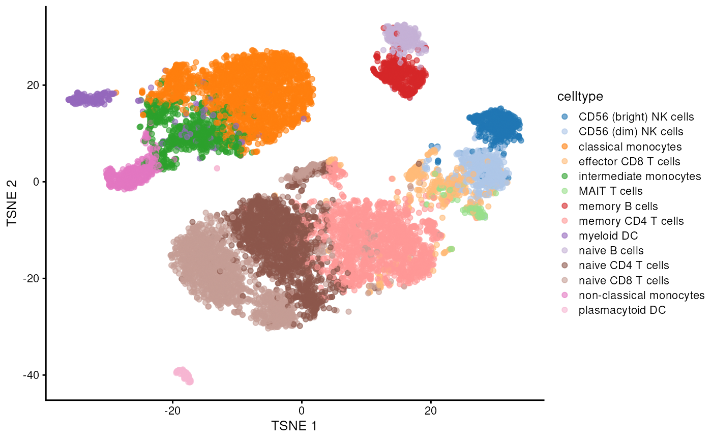
plotReducedDim(sce, dimred = "UMAP", colour_by = "celltype") # Plot UMAP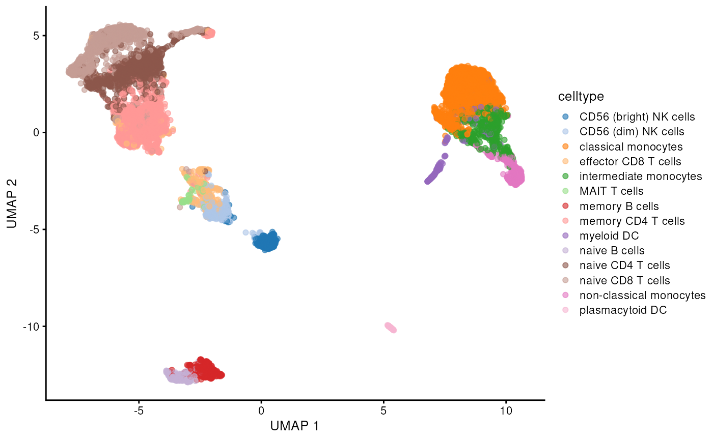
Graph Construction
Construct a shared nearest neighbor (SNN) graph based on PCA-reduced dimensions.
# Build a shared nearest neighbor (SNN) graph
graph <- buildSNNGraph(sce, k = 25, use.dimred = 'PCA')  # k=25 neighbors
Cluster Evaluation
Evaluate different clustering methods using robin
# Simplify the graph and evaluate clustering methods
graph <- igraph::simplify(graph)  # Simplify the graph by removing duplicate edges
Robin
Compare all algorithms vs Louvain
We apply the compare procedure to see which is the algorithm that better fits our network.
graph <- prepGraph(graph, file.format="igraph")
graph <- remove.edge.attribute(graph, "weight")
#Infomap
comp_I <- robinCompare(graph=graph, method1="louvain",
                    method2="infomap")
#Walktrap
comp_W <- robinCompare(graph=graph, method1="louvain",
                       method2="walktrap")
#LabelProp
comp_La <- robinCompare(graph=graph, method1="louvain",
                        method2="labelProp") # use leiden
#Fastgreedy
comp_F <- robinCompare(graph=graph, method1="louvain",
                        method2="fastGreedy")
comp_ll <- robinCompare(graph=graph, method1="louvain",
                        method2="leiden")
path <- system.file("extdata", package = "scrobinv2")
comp_I <- readRDS(file.path(path, "compI.rds"))
comp_W <- readRDS(file.path(path, "compW.rds"))
comp_La <- readRDS(file.path(path, "compLa.rds"))
comp_F <- readRDS(file.path(path, "compF.rds"))
comp_ll <- readRDS(file.path(path, "compll.rds"))
p <- robin::plotMultiCompare(comp_I,comp_W,comp_F,comp_La, comp_ll, title="Robin Compare")
p + labs(color = "Model")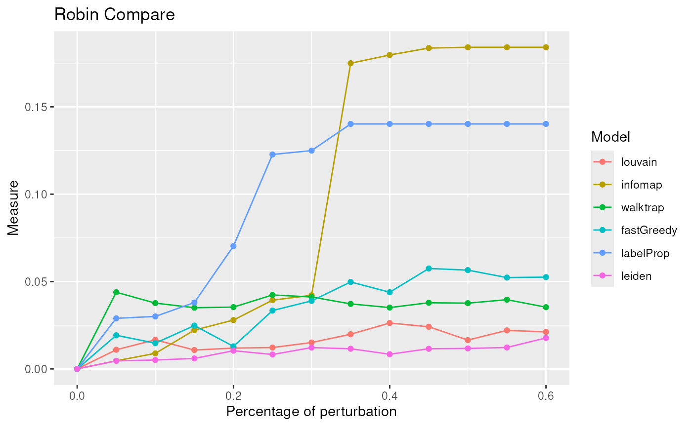
The lowest curve is the most stable algorithm. Leiden and Louvain are the best algorithms in our example.
Statistical significance of communities
Due to the fact that Leiden is one of the best algorithm for our network we apply the robust procedure with the Leiden algorithm to see if the communities detected are statistically significant.
graphRandom <- random(graph=graph)
proc <- robinRobust(graph=graph, graphRandom=graphRandom, method="leiden")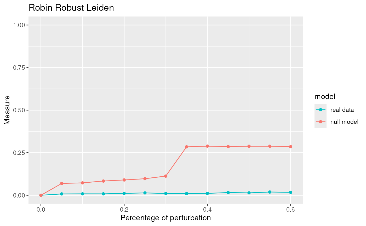
robinFDATest(proc)## [1] "First step: basis expansion"
## Swapping 'y' and 'argvals', because 'y' is simpler,
## and 'argvals' should be; now dim(argvals) = 13 ; dim(y) = 13 x 20
## [1] "Second step: joint univariate tests"
## [1] "Third step: interval-wise combination and correction"
## [1] "creating the p-value matrix: end of row 2 out of 9"
## [1] "creating the p-value matrix: end of row 3 out of 9"
## [1] "creating the p-value matrix: end of row 4 out of 9"
## [1] "creating the p-value matrix: end of row 5 out of 9"
## [1] "creating the p-value matrix: end of row 6 out of 9"
## [1] "creating the p-value matrix: end of row 7 out of 9"
## [1] "creating the p-value matrix: end of row 8 out of 9"
## [1] "creating the p-value matrix: end of row 9 out of 9"
## [1] "Interval Testing Procedure completed"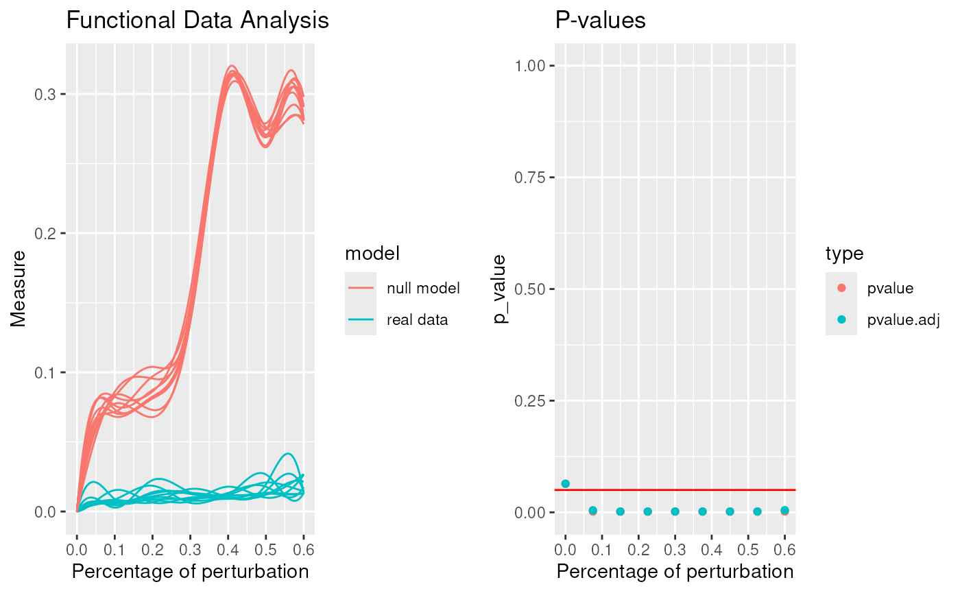
## TableGrob (1 x 2) "arrange": 2 grobs
##   z     cells    name           grob
## 1 1 (1-1,1-1) arrange gtable[layout]
## 2 2 (1-1,2-2) arrange gtable[layout]
## $adj.pvalue
## [1] 0.0640 0.0045 0.0018 0.0018 0.0018 0.0018 0.0018 0.0018 0.0048
##
## $pvalues
## [1] 0.0640 0.0018 0.0018 0.0018 0.0018 0.0018 0.0018 0.0018 0.0018
robinGPTest(proc)## Profile 1
## Profile 2## [1] 105.0276The communities given by Leiden are statistically significant.
Communities
Here we show a table of the number of cells per each community.
mc <- membershipCommunities(graph=graph, method="leiden")
table(mc)
## mc
## 1 2 3 4 5 6 7 8 9 10 11
## 1315 1573 375 2694 150 1067 1227 229 581 715 106Comparing best clustering
To have a complete overview of the obtained results, we now compare the obtained clusters with annotated celltypes by singleR.
To do this kind of analysis, we used as a refernce the
MonacoImmuneData dataset provided by the celldex
bioconductor package.
monacosce <- MonacoImmuneData()

sr <- SingleR(test=sce, ref=monacosce, labels=monacosce$label.fine)

sce$singleR <- sr$labels
We now store the communities into the sce object and use them in combination with the reference to annotate them.
set.seed(999)

sce$leiden <- as.factor(mc)

src <- SingleR(test=sce, ref=monacosce, labels=monacosce$label.fine, clusters=sce$leiden)
names(src$labels) <- names(table(sce$leiden))

sce$singleRLeiden <- NA
for(i in names(src$labels))
{
    sce$singleRLeiden[which(sce$leiden == i)] <- src$labels[i]
}
Here we compare the results obtained between the original cell types and the annotated results using the transformed VI metric.
## Comparison between ground truth and SingleR labels alone
igraph::compare(sce$celltype, sce$singleR, method="vi")/log2(dim(sce)[2])
## [1] 0.1057567
## Comparison between ground truth and Clusters computed with Leiden
igraph::compare(sce$celltype, sce$leiden, method="vi")/log2(dim(sce)[2])
## [1] 0.08023267
## Comparison between ground truth and SingleR with labels + clusters
igraph::compare(sce$celltype, sce$singleRLeiden, method="vi")/log2(dim(sce)[2])
## [1] 0.07341289Finally, to better investigate the results, we plot a heatmap where we have the original cell types on the y axis and the different annotations on the x axis.
# source(system.file("scripts", "functions.R", package = "scrobinv2"))
source(get_data_path("functions.R"))
df <- as.data.frame(colData(sce))
clusterDotPlot(df, "leiden", "celltype")
## [1] "ARI = 0.64"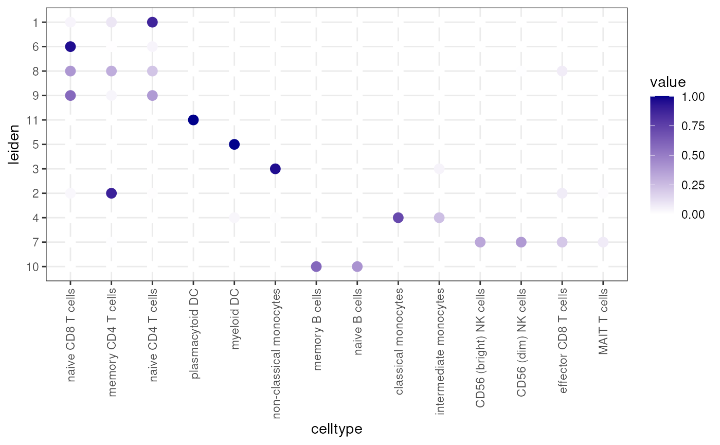
clusterDotPlot(df, "singleR", "celltype")## [1] "ARI = 0.64"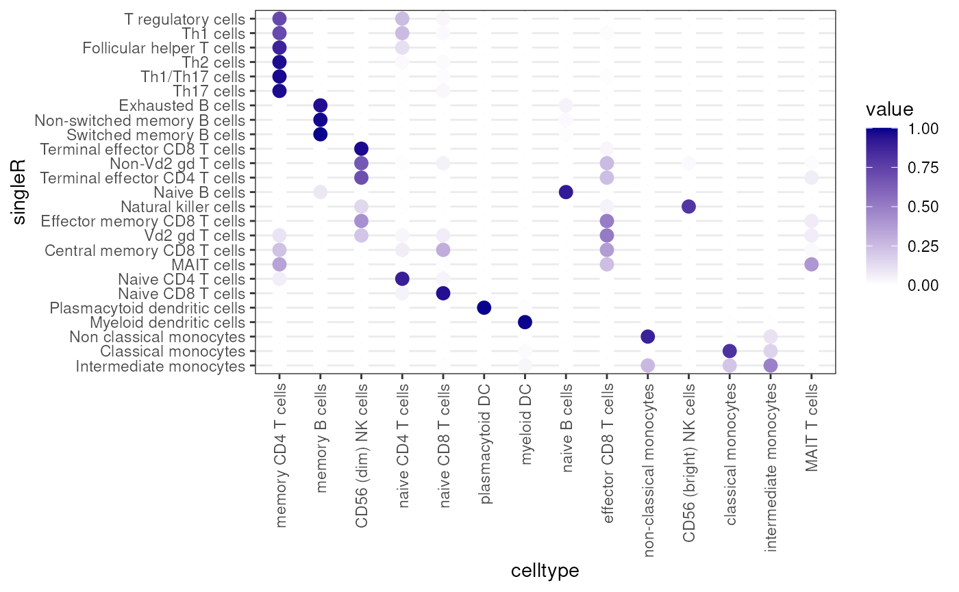
clusterDotPlot(df, "singleRLeiden", "celltype")## [1] "ARI = 0.66"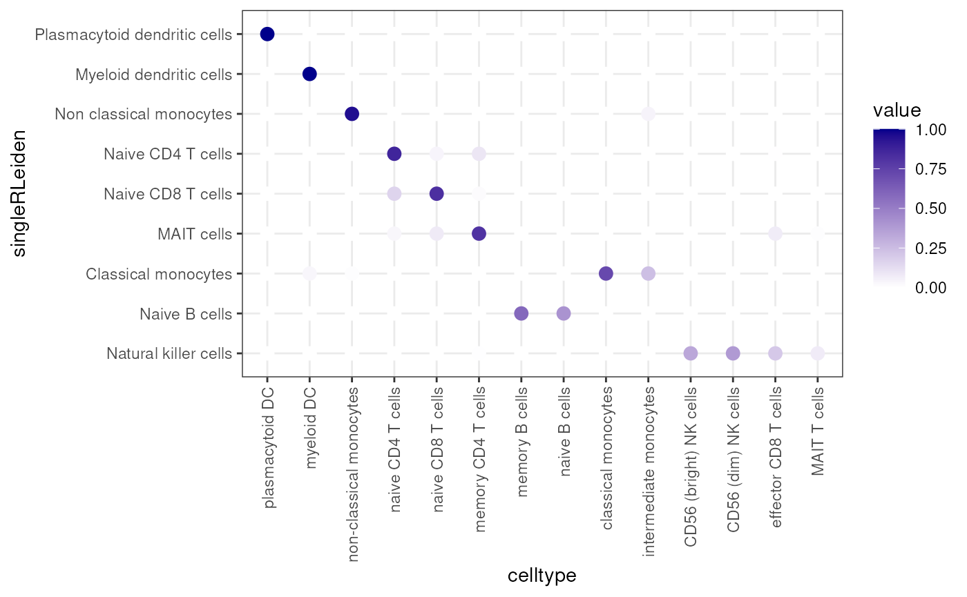
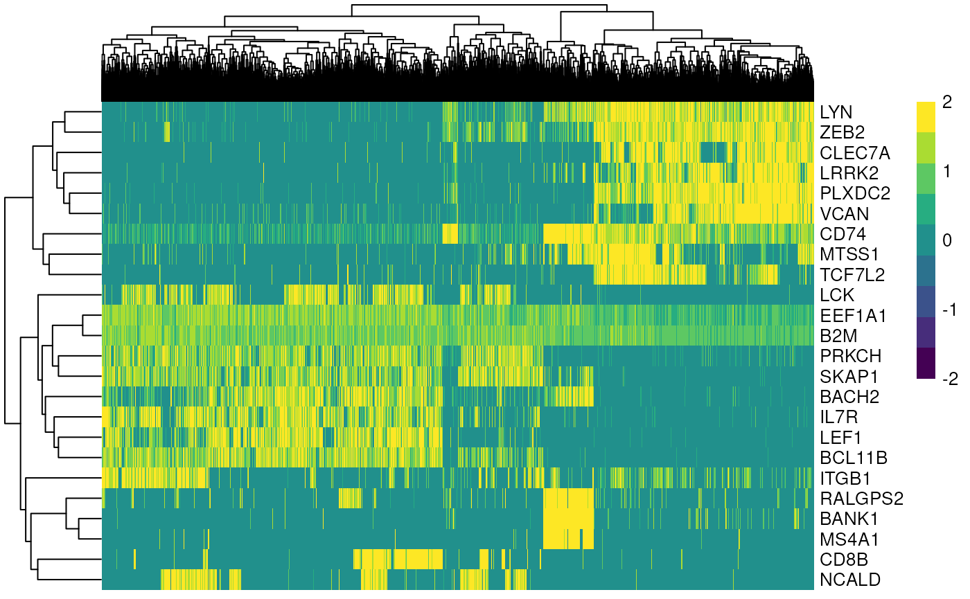
Differential Analysis (Marker Gene Identification)
Once we found the best clustering algorithm, we can use the found communities for identifying marker genes, to subsequently find cell types.
markers <- findMarkers(sce, groups=sce$leiden)
marker_genes <- unique(unlist(lapply(markers, function(m) head(rownames(m), 5))))
plotHeatmap(
  sce,
  features = marker_genes,
  columns_by = "louvain",
  exprs_values = "logcounts",
  scale = TRUE,
  centre = TRUE,
  zlim = c(-2, 2)
)
Session Info
## R version 4.4.2 (2024-10-31)
## Platform: x86_64-pc-linux-gnu
## Running under: Ubuntu 24.04.1 LTS
##
## Matrix products: default
## BLAS:   /usr/lib/x86_64-linux-gnu/openblas-pthread/libblas.so.3
## LAPACK: /usr/lib/x86_64-linux-gnu/openblas-pthread/libopenblasp-r0.3.26.so;  LAPACK version 3.12.0
##
## locale:
##  [1] LC_CTYPE=en_US.UTF-8       LC_NUMERIC=C
##  [3] LC_TIME=en_US.UTF-8        LC_COLLATE=en_US.UTF-8
##  [5] LC_MONETARY=en_US.UTF-8    LC_MESSAGES=en_US.UTF-8
##  [7] LC_PAPER=en_US.UTF-8       LC_NAME=C
##  [9] LC_ADDRESS=C               LC_TELEPHONE=C
## [11] LC_MEASUREMENT=en_US.UTF-8 LC_IDENTIFICATION=C
##
## time zone: Etc/UTC
## tzcode source: system (glibc)
##
## attached base packages:
## [1] stats4    stats     graphics  grDevices utils     datasets  methods
## [8] base
##
## other attached packages:
##  [1] reshape2_1.4.5              robin_2.0.0
##  [3] bluster_1.16.0              celldex_1.16.0
##  [5] SingleR_2.8.0               igraph_2.2.1
##  [7] scran_1.34.0                BiocParallel_1.40.2
##  [9] scater_1.34.1               ggplot2_4.0.1
## [11] scuttle_1.16.0              SingleCellExperiment_1.28.1
## [13] SummarizedExperiment_1.36.0 Biobase_2.66.0
## [15] GenomicRanges_1.58.0        GenomeInfoDb_1.42.3
## [17] IRanges_2.40.1              S4Vectors_0.44.0
## [19] BiocGenerics_0.52.0         MatrixGenerics_1.18.1
## [21] matrixStats_1.5.0
##
## loaded via a namespace (and not attached):
##   [1] splines_4.4.2             bitops_1.0-9
##   [3] filelock_1.0.3            cellranger_1.1.0
##   [5] tibble_3.3.0              deSolve_1.40
##   [7] lifecycle_1.0.4           httr2_1.2.2
##   [9] edgeR_4.4.2               lattice_0.22-7
##  [11] MASS_7.3-65               alabaster.base_1.6.1
##  [13] magrittr_2.0.4            limma_3.62.2
##  [15] sass_0.4.10               rmarkdown_2.30
##  [17] jquerylib_0.1.4           yaml_2.3.11
##  [19] metapod_1.14.0            otel_0.2.0
##  [21] askpass_1.2.1             gld_2.6.8
##  [23] cowplot_1.2.0             DBI_1.2.3
##  [25] RColorBrewer_1.1-3        abind_1.4-8
##  [27] zlibbioc_1.52.0           expm_1.0-0
##  [29] RCurl_1.98-1.17           pracma_2.4.6
##  [31] rappdirs_0.3.3            GenomeInfoDbData_1.2.13
##  [33] data.tree_1.2.0           ggrepel_0.9.6
##  [35] irlba_2.3.5.1             pheatmap_1.0.13
##  [37] dqrng_0.4.1               pkgdown_2.2.0
##  [39] DelayedMatrixStats_1.28.1 codetools_0.2-20
##  [41] DelayedArray_0.32.0       tidyselect_1.2.1
##  [43] UCSC.utils_1.2.0          farver_2.1.2
##  [45] ScaledMatrix_1.14.0       viridis_0.6.5
##  [47] BiocFileCache_2.14.0      jsonlite_2.0.0
##  [49] BiocNeighbors_2.0.1       e1071_1.7-16
##  [51] ks_1.15.1                 systemfonts_1.3.1
##  [53] tools_4.4.2               ragg_1.5.0
##  [55] DescTools_0.99.60         Rcpp_1.1.0
##  [57] glue_1.8.0                gridExtra_2.3
##  [59] SparseArray_1.6.2         xfun_0.54
##  [61] dplyr_1.1.4               HDF5Array_1.34.0
##  [63] gypsum_1.2.0              withr_3.0.2
##  [65] formatR_1.14              BiocManager_1.30.27
##  [67] fastmap_1.2.0             boot_1.3-32
##  [69] rhdf5filters_1.18.1       digest_0.6.39
##  [71] rsvd_1.0.5                R6_2.6.1
##  [73] qpdf_1.4.1                textshaping_1.0.4
##  [75] colorspace_2.1-2          networkD3_0.4.1
##  [77] RSQLite_2.4.5             generics_0.1.4
##  [79] data.table_1.17.8         class_7.3-23
##  [81] httr_1.4.7                htmlwidgets_1.6.4
##  [83] S4Arrays_1.6.0            pkgconfig_2.0.3
##  [85] Exact_3.3                 gtable_0.3.6
##  [87] blob_1.2.4                S7_0.2.1
##  [89] XVector_0.46.0            pcaPP_2.0-5
##  [91] htmltools_0.5.9           scales_1.4.0
##  [93] alabaster.matrix_1.6.1    perturbR_0.1.3
##  [95] lmom_3.2                  png_0.1-8
##  [97] rstudioapi_0.17.1         knitr_1.50
##  [99] tzdb_0.5.0                curl_7.0.0
## [101] proxy_0.4-27              cachem_1.1.0
## [103] rhdf5_2.50.2              stringr_1.6.0
## [105] rootSolve_1.8.2.4         BiocVersion_3.20.0
## [107] KernSmooth_2.23-26        parallel_4.4.2
## [109] fda_6.3.0                 vipor_0.4.7
## [111] AnnotationDbi_1.68.0      desc_1.4.3
## [113] pillar_1.11.1             grid_4.4.2
## [115] alabaster.schemas_1.6.0   vctrs_0.6.5
## [117] BiocSingular_1.22.0       dbplyr_2.5.1
## [119] beachmat_2.22.0           cluster_2.1.8.1
## [121] beeswarm_0.4.0            evaluate_1.0.5
## [123] readr_2.1.6               mvtnorm_1.3-3
## [125] cli_3.6.5                 locfit_1.5-9.12
## [127] compiler_4.4.2            rlang_1.1.6
## [129] crayon_1.5.3              fdatest_2.1.1
## [131] labeling_0.4.3            mclust_6.1.2
## [133] fds_1.8                   plyr_1.8.9
## [135] forcats_1.0.1             fs_1.6.6
## [137] ggbeeswarm_0.7.3          stringi_1.8.7
## [139] rainbow_3.8               viridisLite_0.4.2
## [141] alabaster.se_1.6.0        hdrcde_3.4
## [143] Biostrings_2.74.1         Matrix_1.7-4
## [145] ExperimentHub_2.14.0      hms_1.1.4
## [147] sparseMatrixStats_1.18.0  bit64_4.6.0-1
## [149] Rhdf5lib_1.28.0           KEGGREST_1.46.0
## [151] statmod_1.5.1             haven_2.5.5
## [153] alabaster.ranges_1.6.0    AnnotationHub_3.14.0
## [155] memoise_2.0.1             bslib_0.9.0
## [157] bit_4.6.0                 readxl_1.4.5