STexampleData package

The STexampleData package provides access to several spatially resolved transcriptomics datasets, which have been formatted into the SpatialExperiment Bioconductor class.

These datasets have been collected from various publicly available sources, and cover several technological platforms.

We provide these datasets as SpatialExperiment objects to make them easier to access, so that we and others can use them for examples, demonstrations, tutorials, and other purposes.

Additional datasets from the 10x Genomics Visium platform are also available in the TENxVisiumData package (developed by Helena Crowell).

Datasets

The package currently contains the following datasets:

Visium_humanDLPFC (10x Genomics Visium): A single sample (sample 151673) of human brain dorsolateral prefrontal cortex (DLPFC) in the human brain, measured using the 10x Genomics Visium platform. This is a subset of the full dataset containing 12 samples from 3 neurotypical donors, published by Maynard and Collado-Torres et al. (2021). The full dataset is available from the spatialLIBD Bioconductor package.
Visium_mouseCoronal (10x Genomics Visium): A single coronal section from the mouse brain, spanning one hemisphere. This dataset was previously released by 10x Genomics on their website.
seqFISH_mouseEmbryo (seqFISH): A subset of cells (embryo 1, z-slice 2) from a previously published dataset investigating mouse embryogenesis by Lohoff and Ghazanfar et al. (2020), generated using the seqFISH platform. The full dataset is available online.

Install package

The package can be installed from Bioconductor as follows.

BiocManager::install("STexampleData", version = "devel")

Alternatively, the latest version can also be installed from GitHub. For this workshop, we use the latest development version from GitHub.

remotes::install_github("lmweber/STexampleData", ref = "no_accessors", build_vignettes = TRUE)

Load dataset

First, we check the available datasets from the STexampleData package stored in Bioconductor’s ExperimentHub resource.

# load packages
library(ExperimentHub)

# query ExperimentHub resource
eh <- ExperimentHub()

## snapshotDate(): 2021-05-18

query(eh, "STexampleData")

## ExperimentHub with 3 records
## # snapshotDate(): 2021-05-18
## # $dataprovider: NA
## # $species: Mus musculus, Homo sapiens
## # $rdataclass: SpatialExperiment
## # additional mcols(): taxonomyid, genome, description,
## #   coordinate_1_based, maintainer, rdatadateadded, preparerclass, tags,
## #   rdatapath, sourceurl, sourcetype 
## # retrieve records with, e.g., 'object[["EH5443"]]' 
## 
##            title                   
##   EH5443 | Visium_humanDLPFC_3_13  
##   EH5444 | Visium_mouseCoronal_3_13
##   EH5445 | seqFISH_mouseEmbryo_3_13

Next, we run a short example showing how to load one of the datasets from the STexampleData package.

Alternative ways of loading the datasets from ExperimentHub are shown in the package vignette.

# load packages
library(SpatialExperiment)
library(STexampleData)

# load dataset from latest development version
spe <- load_data("Visium_humanDLPFC")

# alternatively: load from ExperimentHub using named accessor function
# spe <- Visium_humanDLPFC()

Then, we have a look at the structure of the SpatialExperiment object.

spe

## class: SpatialExperiment 
## dim: 33538 4992 
## metadata(0):
## assays(1): counts
## rownames(33538): ENSG00000243485 ENSG00000237613 ... ENSG00000277475
##   ENSG00000268674
## rowData names(3): gene_id gene_name feature_type
## colnames(4992): AAACAACGAATAGTTC-1 AAACAAGTATCTCCCA-1 ...
##   TTGTTTGTATTACACG-1 TTGTTTGTGTAAATTC-1
## colData names(3): cell_count ground_truth sample_id
## reducedDimNames(0):
## mainExpName: NULL
## altExpNames(0):
## spatialData names(6) : barcode_id in_tissue ... pxl_col_in_fullres
##   pxl_row_in_fullres
## spatialCoords names(2) : x y
## imgData names(4): sample_id image_id data scaleFactor

dim(spe)

## [1] 33538  4992

assayNames(spe)

## [1] "counts"

rowData(spe)

## DataFrame with 33538 rows and 3 columns
##                         gene_id   gene_name    feature_type
##                     <character> <character>     <character>
## ENSG00000243485 ENSG00000243485 MIR1302-2HG Gene Expression
## ENSG00000237613 ENSG00000237613     FAM138A Gene Expression
## ENSG00000186092 ENSG00000186092       OR4F5 Gene Expression
## ENSG00000238009 ENSG00000238009  AL627309.1 Gene Expression
## ENSG00000239945 ENSG00000239945  AL627309.3 Gene Expression
## ...                         ...         ...             ...
## ENSG00000277856 ENSG00000277856  AC233755.2 Gene Expression
## ENSG00000275063 ENSG00000275063  AC233755.1 Gene Expression
## ENSG00000271254 ENSG00000271254  AC240274.1 Gene Expression
## ENSG00000277475 ENSG00000277475  AC213203.1 Gene Expression
## ENSG00000268674 ENSG00000268674     FAM231C Gene Expression

colData(spe)

## DataFrame with 4992 rows and 3 columns
##                    cell_count ground_truth     sample_id
##                     <integer>     <factor>   <character>
## AAACAACGAATAGTTC-1         NA       NA     sample_151673
## AAACAAGTATCTCCCA-1          6       Layer3 sample_151673
## AAACAATCTACTAGCA-1         16       Layer1 sample_151673
## AAACACCAATAACTGC-1          5       WM     sample_151673
## AAACAGAGCGACTCCT-1          2       Layer3 sample_151673
## ...                       ...          ...           ...
## TTGTTTCACATCCAGG-1          3       WM     sample_151673
## TTGTTTCATTAGTCTA-1          4       WM     sample_151673
## TTGTTTCCATACAACT-1          3       Layer6 sample_151673
## TTGTTTGTATTACACG-1         16       WM     sample_151673
## TTGTTTGTGTAAATTC-1          5       Layer2 sample_151673

spatialData(spe)

## DataFrame with 4992 rows and 6 columns
##                            barcode_id in_tissue array_row array_col
##                           <character> <integer> <integer> <integer>
## AAACAACGAATAGTTC-1 AAACAACGAATAGTTC-1         0         0        16
## AAACAAGTATCTCCCA-1 AAACAAGTATCTCCCA-1         1        50       102
## AAACAATCTACTAGCA-1 AAACAATCTACTAGCA-1         1         3        43
## AAACACCAATAACTGC-1 AAACACCAATAACTGC-1         1        59        19
## AAACAGAGCGACTCCT-1 AAACAGAGCGACTCCT-1         1        14        94
## ...                               ...       ...       ...       ...
## TTGTTTCACATCCAGG-1 TTGTTTCACATCCAGG-1         1        58        42
## TTGTTTCATTAGTCTA-1 TTGTTTCATTAGTCTA-1         1        60        30
## TTGTTTCCATACAACT-1 TTGTTTCCATACAACT-1         1        45        27
## TTGTTTGTATTACACG-1 TTGTTTGTATTACACG-1         1        73        41
## TTGTTTGTGTAAATTC-1 TTGTTTGTGTAAATTC-1         1         7        51
##                    pxl_col_in_fullres pxl_row_in_fullres
##                             <integer>          <integer>
## AAACAACGAATAGTTC-1               2435               3913
## AAACAAGTATCTCCCA-1               8468               9791
## AAACAATCTACTAGCA-1               2807               5769
## AAACACCAATAACTGC-1               9505               4068
## AAACAGAGCGACTCCT-1               4151               9271
## ...                               ...                ...
## TTGTTTCACATCCAGG-1               9396               5653
## TTGTTTCATTAGTCTA-1               9630               4825
## TTGTTTCCATACAACT-1               7831               4631
## TTGTTTGTATTACACG-1              11193               5571
## TTGTTTGTGTAAATTC-1               3291               6317

head(spatialCoords(spe))

##                       x    y
## AAACAACGAATAGTTC-1 3913 2435
## AAACAAGTATCTCCCA-1 9791 8468
## AAACAATCTACTAGCA-1 5769 2807
## AAACACCAATAACTGC-1 4068 9505
## AAACAGAGCGACTCCT-1 9271 4151
## AAACAGCTTTCAGAAG-1 3393 7583

imgData(spe)

## DataFrame with 2 rows and 4 columns
##       sample_id    image_id   data scaleFactor
##     <character> <character> <list>   <numeric>
## 1 sample_151673      lowres   ####   0.0450045
## 2 sample_151673       hires   ####   0.1500150

Plot dataset

Next, we generate some simple plots of the dataset. We can use plotting functions available in the ggspavis package, which is available from GitHub.

# install ggspavis package
remotes::install_github("lmweber/ggspavis", build_vignettes = TRUE)

# load packages
library(ggspavis)

Create some plots of the dataset in x-y coordinates. This dataset contains a set of manually annotated ground truth labels for cortical layers in the human brain, which we can use to display annotation on the plot.

# plot spots only
plotSpots(spe)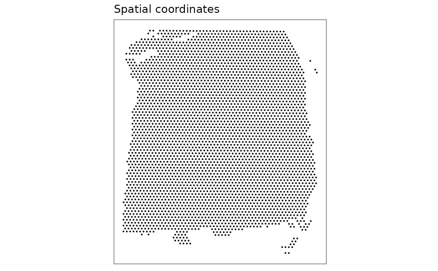

# plot spots with annotation
plotSpots(spe, annotate = "ground_truth")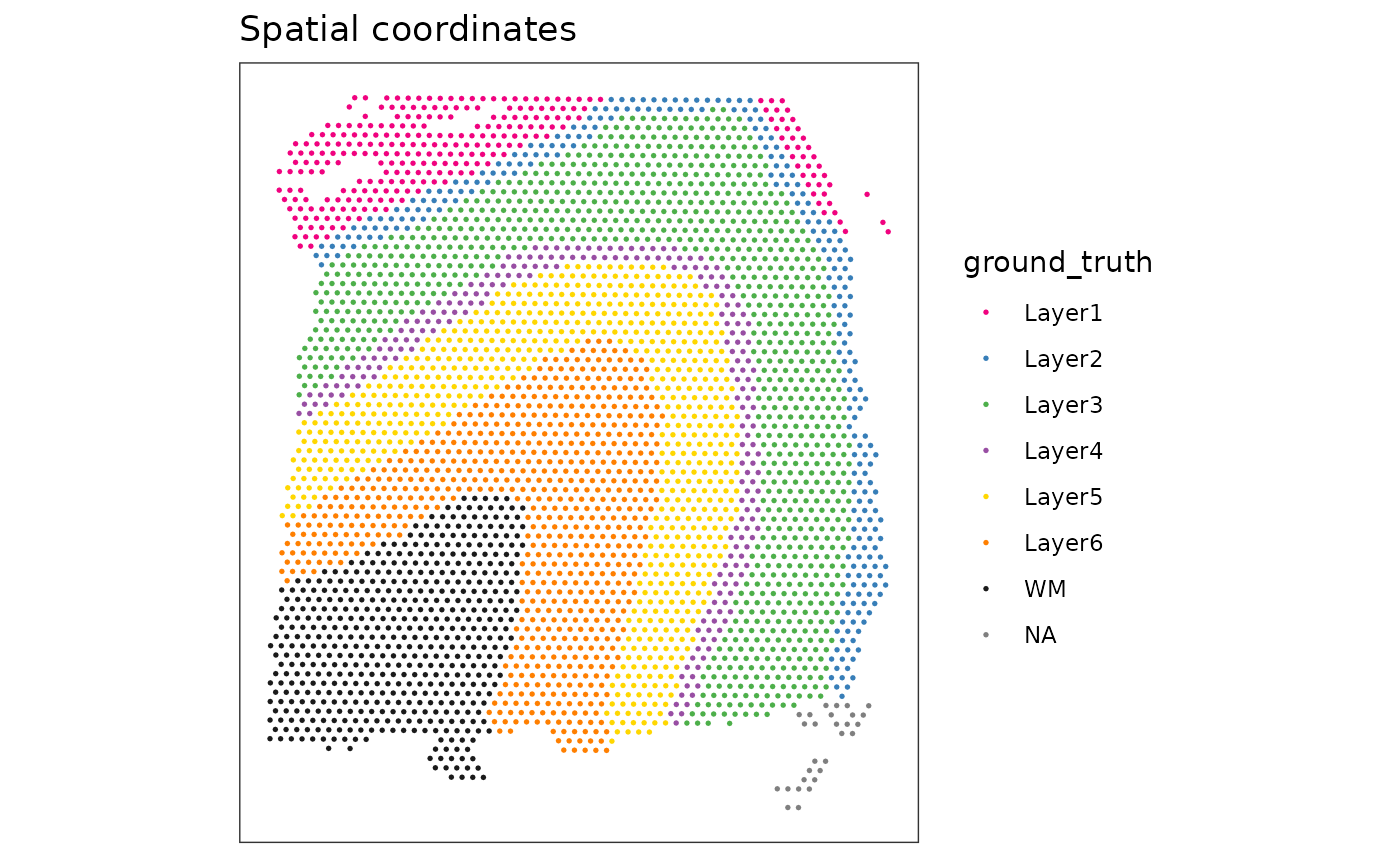

We can also use a more flexible plotting function to display the spots and annotation along with the histology image as background, which is stored in the SpatialExperiment object. We also highlight spots located over tissue, which are identified with the “in_tissue” column in the spatialData.

# plots with histology background
plotVisium(spe)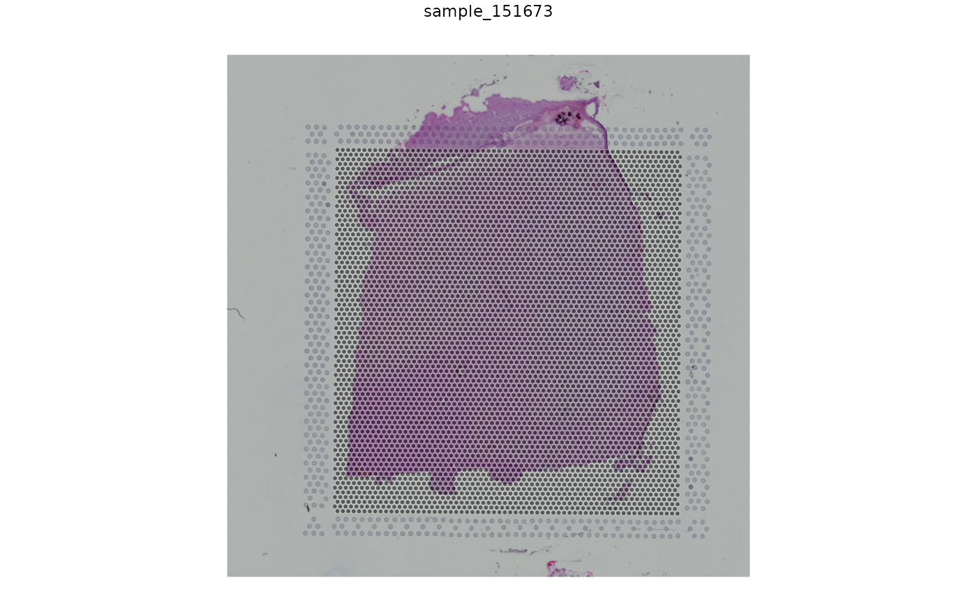

plotVisium(spe, fill = "ground_truth", highlight = "in_tissue")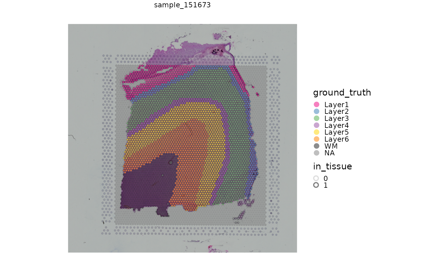

Exercise

For some additional practice with these objects, attempt the following:

Generate a plot in x-y coordinates with annotation showing total unique molecular identifier (UMI) counts
Generate a plot in x-y coordinates with annotation showing expression of a specific gene of interest, e.g. SNAP25, MOBP, or PCP4

You can refer to the help files for the plotting functions with ?plotSpots and ?plotVisium.

For a further exercise, try adjusting the color palettes and other plotting options, as described in the help files.