Reading 10X Visium data

The 10X Genomics’ Space Ranger pipeline will process data using standard output file formats that are saved, for each sample, in a single directory /<sample>/outs/ of the following structure:

sample
|—outs 
··|—raw/filtered_feature_bc_matrix.h5
··|—raw/filtered_feature_bc_matrix
····|—barcodes.tsv
····|—features.tsv
····|—matrix.mtx
··|—spatial
····|—tissue_hires_image.png
····|—tissue_lowres_image.png
····|—detected_tissue_image.jpg
····|—aligned_fiducials.jpg
····|—scalefactors_json.json
····|—tissue_positions_list.csv

The SpatialExperiment package provides an exemplary 10X Visium spatial gene expression data of two serial mouse brain sections (Sagittal-Posterior) available from the 10X Genomics website. These are located in the extdata/10xVisium directory:

library(SpatialExperiment)

dir <- system.file(
  file.path("extdata", "10xVisium"),
  package = "SpatialExperiment")

sample_ids <- c("section1", "section2")
samples <- file.path(dir, sample_ids)

We can load these data into a SpatialExperiment using the read10xVisium() function, which will read in all relevant information, including the count data, spatial metadata and coordinates, scale factors, and images:

list.files(samples[1])

## [1] "raw_feature_bc_matrix" "spatial"

list.files(file.path(samples[1], "spatial"))

## [1] "scalefactors_json.json"    "tissue_lowres_image.png"  
## [3] "tissue_positions_list.csv"

(spe <- read10xVisium(samples, sample_ids,
  type = "sparse",   # use sparse (not HDF5) format
  data = "raw",      # read all (not filtered) data
  images = "lowres", # specify which image(s) to include
  load = TRUE))      # specify whether or not to load image(s)

## class: SpatialExperiment 
## dim: 50 99 
## metadata(0):
## assays(1): counts
## rownames(50): ENSMUSG00000051951 ENSMUSG00000089699 ...
##   ENSMUSG00000005886 ENSMUSG00000101476
## rowData names(1): symbol
## colnames(99): AAACAACGAATAGTTC-1 AAACAAGTATCTCCCA-1 ...
##   AAAGTCGACCCTCAGT-1 AAAGTGCCATCAATTA-1
## colData names(1): sample_id
## reducedDimNames(0):
## mainExpName: NULL
## altExpNames(0):
## spatialData names(3) : in_tissue array_row array_col
## spatialCoords names(2) : pxl_col_in_fullres pxl_row_in_fullres
## imgData names(4): sample_id image_id data scaleFactor

The `SpatialExperiment` class

`spatialData` & `-Coords`

Spatial metadata are stored inside the int_colData’s spatialData field as a DataFrame and include:

in_tissue indicating whether an observation was mapped to tissue
array_row/col giving the spots’ row/column coordinate in the array¹

head(spatialData(spe))

## DataFrame with 6 rows and 3 columns
##                    in_tissue array_row array_col
##                    <logical> <integer> <integer>
## AAACAACGAATAGTTC-1     FALSE         0        16
## AAACAAGTATCTCCCA-1      TRUE        50       102
## AAACAATCTACTAGCA-1      TRUE         3        43
## AAACACCAATAACTGC-1      TRUE        59        19
## AAACAGAGCGACTCCT-1      TRUE        14        94
## AAACAGCTTTCAGAAG-1     FALSE        43         9

# tabulate number of spots mapped to tissue
table(
    sample_id = spe$sample_id,
    in_tissue = spatialData(spe)$in_tissue)

##           in_tissue
## sample_id  FALSE TRUE
##   section1    28   22
##   section2    27   22

A numeric matrix of spatial coordinates (here, x and y) is stored inside the int_colData’s spatialCoords field, and can be accessed using the spatialCoords() accessor:

head(spatialCoords(spe))

##                    pxl_col_in_fullres pxl_row_in_fullres
## AAACAACGAATAGTTC-1               1252               2312
## AAACAAGTATCTCCCA-1               7237               8230
## AAACAATCTACTAGCA-1               1611               4170
## AAACACCAATAACTGC-1               8315               2519
## AAACAGAGCGACTCCT-1               2927               7679
## AAACAGCTTTCAGAAG-1               6400               1831

Note that the colData, spatialData, and spatialCoords slots follow a hierarchical structure where colData > spatialData > spatialCoords. Here, each accessor function allows joint accession of the target slot, and (optionally) any slot(s) that precedes it.

Specifically, the following commands are supported may be used to access specific subsets of (spatial) metadata associated with each column (observation, e.g. spots or cells) in a SPE:

spatialCoords(spe)

spatialData(spe)
spatialData(spe, spatialCoords = TRUE)

colData(spe, spatialData = TRUE)
colData(spe, spatialCoords = TRUE)
colData(spe, spatialData = TRUE, spatialCoords = TRUE)

`imgData`

Image-related data are stored in the int_metadata’s imgData field as a DataFrame with the following columns:

sample_id and image_id specifying the image’s sample and image identifier
data is a list of SpatialImages containing the image’s grob, path and/or URL
scaleFactors are used to rescale spatial coordinates according to the image’s resolution

We can retrieve these data using the imgData() accessor:

imgData(spe)

## DataFrame with 2 rows and 4 columns
##     sample_id    image_id   data scaleFactor
##   <character> <character> <list>   <numeric>
## 1    section1      lowres   ####   0.0510334
## 2    section2      lowres   ####   0.0510334

The `SpatialImage` class

Images inside a SpatialExperiment’s imgData are stored as objects of class SpatialImage. The SpatialImage class hierarchy provides representations of images from a variety of sources, including:

LoadedSpatialImage: an image that is fully realized into memory, where the raster representation is stored inside the output object.
RemoteSpatialImage: an image that is remotely hosted and retrieved only on request.
StoredSpatialImage: an image that is stored in a local file and is loaded into memory only on request.

A list of SpatialImages can be retrieved from the imgData’s data field using the $ accessor:

imgData(spe)$data

## [[1]]
## A 600 x 576 LoadedSpatialImage 
## 
## [[2]]
## A 600 x 576 LoadedSpatialImage

For StoredSpatialImage and RemoteSpatialImage objects, loading the image with imgRaster() (see next section) will automatically store the loaded raster object in an in-memory cache. Any subsequent imgRaster() call will retrieve the raster from the cache, avoiding costly retrieval from the file system.

This provides the option to store an image’s source at minimal storage cost, which is desirable when multiple images are to be stored (say, for many samples and of different resolutions), or when a SpatialExperiment is to be exported.

Methods for image handling

The SpatialExperiment package provides various functions to handle which and how image data is stored in the object. These include:

get/add/rmvImg to retrieve/add/remove (an) image(s) from a SpatialExperiment
imgSource/Raster to retrieve the path/URL or raster object associated with (an) image(s)

get/rmvImg() and imgSource/Raster() are flexible in the specification of the sample/image_id arguments. Specifically,

TRUE is equivalent to all, e.g. sample_id = "<sample>", image_id = TRUE will drop all images for a given sample.
NULL defaults to the first entry available, e.g., sample_id = "<sample>", image_id = NULL will drop the first image for a given sample.

For example, sample_id,image_id = TRUE,TRUE will specify all images; NULL,NULL corresponds to the first image entry in the imgData; TRUE,NULL equals the first image for all samples; and NULL,TRUE matches all images for the first sample.

`raster` & source accession

Data available in an object of class SpatialImage may be accessed via the imgRaster() and imgSource() accessors. Note that, since our images are LoadedSpatialImages, there source is NA:

si <- imgData(spe)$data[[1]]
head(imgRaster(si)[, 1:4])

##      [,1]        [,2]        [,3]        [,4]       
## [1,] "#82847fff" "#81847fff" "#81847fff" "#81847fff"
## [2,] "#81847fff" "#81847fff" "#81847eff" "#81847fff"
## [3,] "#82847fff" "#82847fff" "#828580ff" "#81857fff"
## [4,] "#828580ff" "#82847fff" "#82857fff" "#82847fff"
## [5,] "#82847fff" "#828580ff" "#828580ff" "#828580ff"
## [6,] "#82857fff" "#828480ff" "#82847fff" "#828480ff"

imgSource(si)

## [1] NA

Using as.raster() or, equivalently, the imgRaster() accessor, a SpatialImage may be converted to a raster object, which can be used directly for plotting:

img1 <- as.raster(si)
img2 <- imgRaster(si)
identical(img1, img2)

## [1] TRUE

par(mar = c(0,0,0,0))
plot(img1)

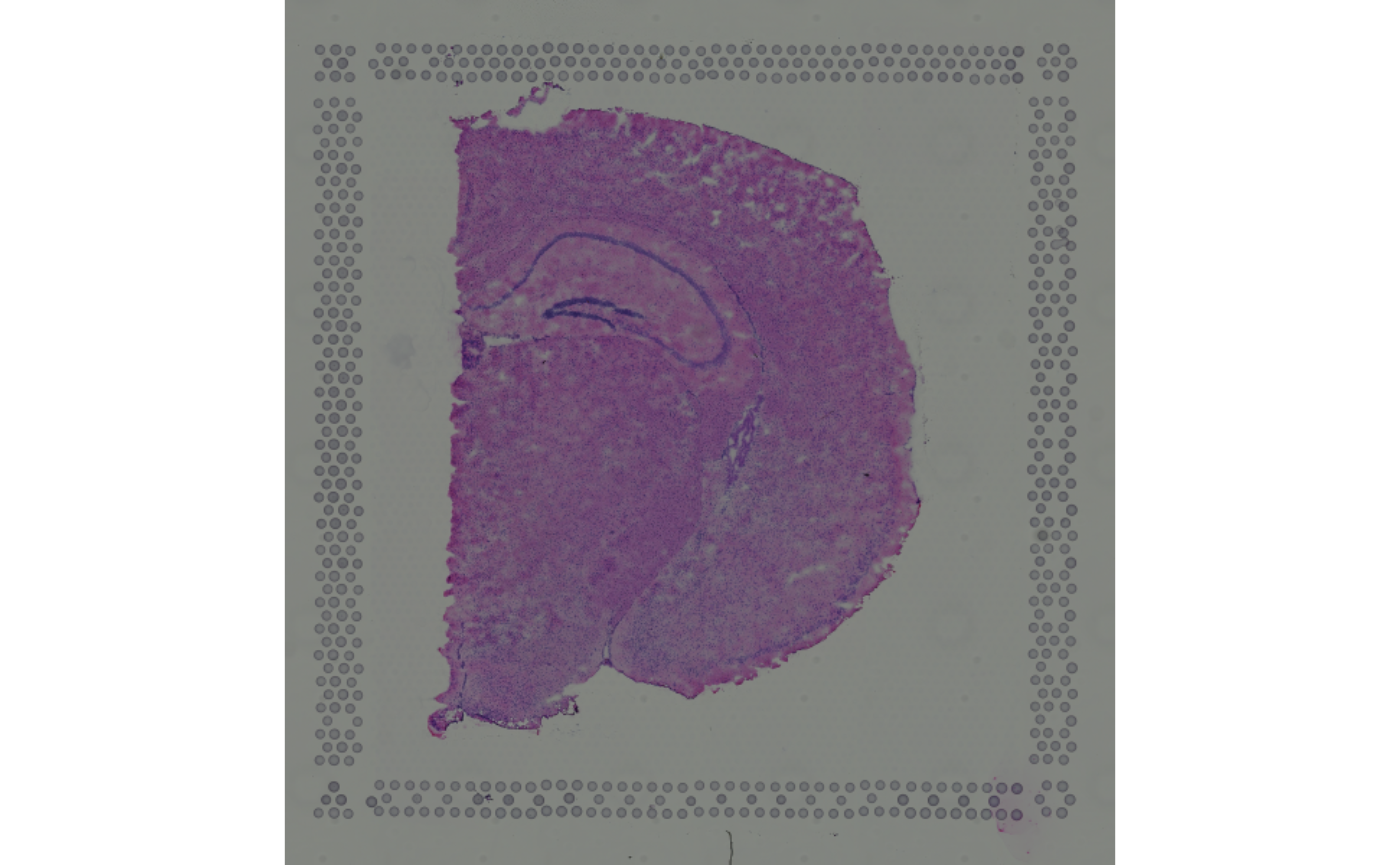
In the example below, we access all images as raster objects (via setting sample_id = image_id = TRUE):

imgs <- imgRaster(spe, sample_id = TRUE, image_id = TRUE)
sapply(imgs, \(.) c(dim = dim(.), class = class(.)))

##       [,1]     [,2]    
## dim1  "600"    "600"   
## dim2  "576"    "576"   
## class "raster" "raster"

Adding & removing images

Besides a path or URL to source the image from and a numeric scale factor, addImg() requires specification of the sample_id the new image belongs to, and an image_id that is not yet in use for that sample:

url <- "https://i.redd.it/3pw5uah7xo041.jpg"
spe <- addImg(spe,
    sample_id = "section1", 
    image_id = "pomeranian",
    imageSource = url, 
    scaleFactor = NA_real_, 
    load = TRUE)

The above code chunk has added an new image entry in the input SpatialExperiment’s imgData field:

imgData(spe)

## DataFrame with 3 rows and 4 columns
##     sample_id    image_id   data scaleFactor
##   <character> <character> <list>   <numeric>
## 1    section1      lowres   ####   0.0510334
## 2    section2      lowres   ####   0.0510334
## 3    section1  pomeranian   ####          NA

img <- imgRaster(spe,
    sample_id = "section1",
    image_id = "pomeranian")
plot(img)

We can remove specific images with rmvImg():

spe <- rmvImg(spe,
    sample_id = "section1",
    image_id = "pomeranian")
imgData(spe)

## DataFrame with 2 rows and 4 columns
##     sample_id    image_id   data scaleFactor
##   <character> <character> <list>   <numeric>
## 1    section1      lowres   ####   0.0510334
## 2    section2      lowres   ####   0.0510334

`sample_id` replacement

While storing of sample_ids inside the SpatialExperiment’s colData enables direct accessibility via the colData and $ accessors, this field is protected against arbitrary modification. This affects operations to the following effects:

Empty replacement will retain sample identifiers:

tmp <- spe$sample_id
spe$sample_id <- NULL
identical(tmp, spe$sample_id)

## [1] TRUE

Replacement of sample_ids is permitted provided that

the number of unique sample identifiers is retained
newly provided sample identifiers are a one-to-one mapping

spe$sample_id <- sample(c("a", "b", "c"), ncol(spe), TRUE)

## Error in .local(x, ..., value): Number of unique 'sample_id's is 2, but 3 were provided.

spe$sample_id <- sample(c("a", "b"), ncol(spe), TRUE)

## Error in .local(x, ..., value): New 'sample_id's must map uniquely

Valid replacement will be propagated to the imgData:

tmp <- spe
i <- as.numeric(factor(spe$sample_id))
tmp$sample_id <- c("sampleA", "sampleB")[i]
imgData(tmp)

## DataFrame with 2 rows and 4 columns
##     sample_id    image_id   data scaleFactor
##   <character> <character> <list>   <numeric>
## 1     sampleA      lowres   ####   0.0510334
## 2     sampleB      lowres   ####   0.0510334

Session info

sessionInfo()

## R version 4.1.0 (2021-05-18)
## Platform: x86_64-pc-linux-gnu (64-bit)
## Running under: Ubuntu 20.04.2 LTS
## 
## Matrix products: default
## BLAS/LAPACK: /usr/lib/x86_64-linux-gnu/openblas-pthread/libopenblasp-r0.3.8.so
## 
## locale:
##  [1] LC_CTYPE=en_US.UTF-8       LC_NUMERIC=C              
##  [3] LC_TIME=en_US.UTF-8        LC_COLLATE=en_US.UTF-8    
##  [5] LC_MONETARY=en_US.UTF-8    LC_MESSAGES=C             
##  [7] LC_PAPER=en_US.UTF-8       LC_NAME=C                 
##  [9] LC_ADDRESS=C               LC_TELEPHONE=C            
## [11] LC_MEASUREMENT=en_US.UTF-8 LC_IDENTIFICATION=C       
## 
## attached base packages:
## [1] parallel  stats4    stats     graphics  grDevices utils     datasets 
## [8] methods   base     
## 
## other attached packages:
##  [1] SpatialExperiment_1.3.3     SingleCellExperiment_1.14.1
##  [3] SummarizedExperiment_1.22.0 Biobase_2.52.0             
##  [5] GenomicRanges_1.44.0        GenomeInfoDb_1.28.1        
##  [7] IRanges_2.26.0              S4Vectors_0.30.0           
##  [9] BiocGenerics_0.38.0         MatrixGenerics_1.4.2       
## [11] matrixStats_0.60.0         
## 
## loaded via a namespace (and not attached):
##  [1] Rcpp_1.0.7                locfit_1.5-9.4           
##  [3] lattice_0.20-44           rprojroot_2.0.2          
##  [5] digest_0.6.27             R6_2.5.0                 
##  [7] evaluate_0.14             highr_0.9                
##  [9] sparseMatrixStats_1.4.2   zlibbioc_1.38.0          
## [11] rlang_0.4.11              curl_4.3.2               
## [13] jquerylib_0.1.4           magick_2.7.2             
## [15] R.utils_2.10.1            R.oo_1.24.0              
## [17] Matrix_1.3-4              rmarkdown_2.10           
## [19] pkgdown_1.6.1             textshaping_0.3.5        
## [21] desc_1.3.0                BiocParallel_1.26.1      
## [23] stringr_1.4.0             RCurl_1.98-1.3           
## [25] beachmat_2.8.1            DelayedArray_0.18.0      
## [27] HDF5Array_1.20.0          compiler_4.1.0           
## [29] xfun_0.25                 DropletUtils_1.12.2      
## [31] systemfonts_1.0.2         htmltools_0.5.1.1        
## [33] GenomeInfoDbData_1.2.6    edgeR_3.34.0             
## [35] crayon_1.4.1              rhdf5filters_1.4.0       
## [37] bitops_1.0-7              R.methodsS3_1.8.1        
## [39] grid_4.1.0                jsonlite_1.7.2           
## [41] magrittr_2.0.1            dqrng_0.3.0              
## [43] stringi_1.7.3             cachem_1.0.5             
## [45] scuttle_1.2.1             XVector_0.32.0           
## [47] fs_1.5.0                  limma_3.48.3             
## [49] bslib_0.2.5.1             DelayedMatrixStats_1.14.2
## [51] ragg_1.1.3                Rhdf5lib_1.14.2          
## [53] rjson_0.2.20              tools_4.1.0              
## [55] fastmap_1.1.0             yaml_2.2.1               
## [57] rhdf5_2.36.0              memoise_2.0.0            
## [59] knitr_1.33                sass_0.4.0

array_rows range from 0-77 (78 rows); array_cols are even in 0-126 for even rows, and odd in 1-127 for odd rows (64 columns), giving in $78 \times 64 = 4,992$ spots per sample.↩︎

2. The SpatialExperiment class

Helena L. Crowell

Reading 10X Visium data

The `SpatialExperiment` class

`spatialData` & `-Coords`

`imgData`

The `SpatialImage` class

Methods for image handling

`raster` & source accession

Adding & removing images

`sample_id` replacement

Session info

2. The SpatialExperiment class

Helena L. Crowell

Reading 10X Visium data

The SpatialExperiment class

spatialData & -Coords

imgData

The SpatialImage class

Methods for image handling

raster & source accession

Adding & removing images

sample_id replacement

Session info

The `SpatialExperiment` class

`spatialData` & `-Coords`

`imgData`

The `SpatialImage` class

`raster` & source accession

`sample_id` replacement